

The scarfs and gloves come out of the closet.
The neighborhood Starbucks coffee cups change red.
It’s a reminder that autumn is ending.
It’s a reminder that 4 pm is 8 pm.
It’s a reminder that winter is coming.

Today’s temperature in New York is below 30F – a cold November day.
- Do you want to know what the probability of a cold November day is?
- Do you want to know what the return period of such an event is?
- Do you want to know how many such events happened in the last five years?
Get yourself some warm tea. Let the room heater crackle. We’ll dive into rest of the discrete distributions in R.
Get the Data
The National Center for Environmental Information (NCEI) archives weather day for most of the United States. I requested temperature data for Central Park, NYC. Anyone can go online and submit requests for data. They will deliver it to your email in your preferred file format. I filtered the data for our lesson. You can get it from here.
Preliminary Analysis
You can use the following line to read the data file into R workspace.
# Read the temperature data file #
temperature_data = read.table("temperature_data_CentralPark.txt",header=T)
The data has six columns. The first three columns indicate the year, month and day of the record. The fourth, fifth and sixth columns provide the data for average daily temperature, maximum daily temperature, and minimum daily temperature. We will work with the average daily temperature data.
Next, I want to choose the coldest day in November for all the years in the record. For this, I will look through each year’s November data, identify the day with lowest average daily temperature and store it in a matrix. You can use the following lines to get this subset data.
# Years #
years = unique(temperature_data$Year) # Identifying unique years in the data
nyrs = length(years) # number of years of data

# November Coldest Day #
november_coldtemp = matrix(NA,nrow=nyrs,ncol=1)

for (i in 1:nyrs)
{
 days = which((temperature_data$Year==years[i]) & (temperature_data$Month==11)) # index to find november days in each year
 november_coldtemp[i,1] = min(temperature_data$TAVG[days]) # computing the minimum of these days
}
Notice how I am using the which command to find values.
When I plot the data, I notice that there is a long-term trend in the temperature data. In later lessons, we will learn about identifying trends and their causes. For now, let’s take recent data from 1982 – 2016 to avoid the issues that come with the trend.
# Plot the time series #
plot(years, november_coldtemp,type="o")
# There is trend in the data #

# Take a subset of data from recent years to avoid issues with trend (for now)-- #
# 1982 - 2016
november_recent_coldtemp = november_coldtemp[114:148]
plot(1982:2016,november_recent_coldtemp,type="o")
Geometric Distribution
In lesson 33, we learned that the number of trials to the first success is Geometric distribution.
If we consider independent Bernoulli trials of 0s and 1s with some probability of occurrence p and assume X to be a random variable that measures the number of trials it takes to see the first success, then, X is said to be Geometrically distributed.
In our example, the independent Bernoulli trials are years. Each year can have a cold November day (if the lowest November temperature in that year is less than 30F) or not.
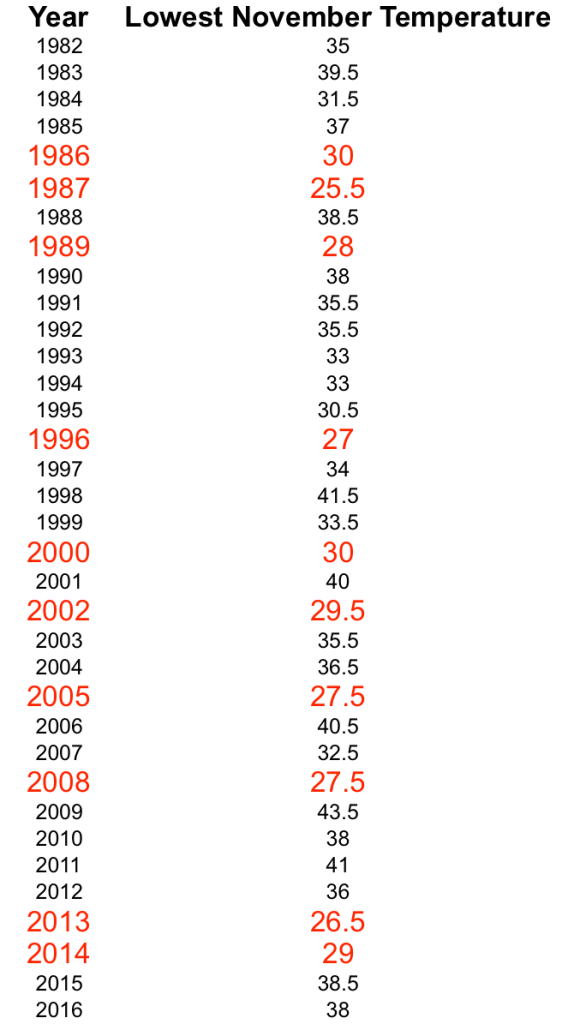
The probability of occurrence is the probability of experiencing a cold November day. A simple estimate of this probability can be obtained by counting the number of years that had a temperature < 30F and dividing this number by the total sample size. In our restricted example, we chose 35 years of data (1982 – 2016) in which we see ten years with lowest November temperature less than 30F. You can see them in the following table.
Success (Cold November) can happen in the first year, in which case X will be 1. We can see the success in the second year, in which case the sequence will be 01, and X will be 2 and so on.
In R, we can compute the probability P(X=1), P(X=2), etc., using the command dgeom. The Inputs are X and p. Try the following lines to create a visual of the distribution.
######################### GEOMETRIC DISTRIBUTION #########################

# The real data case #
n = length(november_recent_coldtemp)

cold_years = which(november_recent_coldtemp <= 30)

ncold = length(cold_years)

p = ncold/n

x = 0:n
px = dgeom(x,p)
plot((x+1),px,type="h",xlab="Random Variable X (Cold on kth year)",ylab="Probability P(X=k)",font=2,font.lab=2)
abline(v = (1/p),col="red",lwd=2)
txt1 = paste("probability of cold year (p) = ",round(p,2),sep="")
txt2 = paste("Return period of cold years = E[X] = 1/p ~ 3.5 years",sep="")
text(20,0.2,txt1,col="red",cex=1)
text(20,0.1,txt2,col="red",cex=1)

Notice the geometric decay in the distribution. It can take X years to see the first success (or the next success from the current success). You must have seen that I have a thick red line at 3.5 years. This is the expected value of the geometric distribution. In lesson 34, we learned that the expected value of the geometric distribution is the return period of the event. On average, how many years does it take before we see the cold year again?
Did we answer the first two questions?
- Do you want to know what the probability of a cold November day is?
- Do you want to know what the return period of such an event is?
Suppose we want to compute the probability that the first success will occur within the next five years, we can use the command pgeom for this purpose.
pgeom computes P(X < 5) as P(X = 1) + P(X = 2) + P(X=3) + P(X = 4). Try it for yourself and verify that they both match.
Suppose the probability is higher or lower, how do you think the distribution will change?
For this, I created an animation of the geometric distribution with changing values of p. See how the distribution is wider for smaller values of p and steeper for larger values of p. A high value of p (probability of the cold November year) indicates that the event will occur more often; hence the trials to success are less in number. On the other hand, a smaller value for p suggests that the event will occur less frequently. The number of trials it takes to see the first/next success is more; creating a wider distribution.
Here is the code for creating the animation. We used similar code last week for animating the binomial distribution.
######## Animation (varying p) #########
# Create png files for Geometric distribution #

png(file="geometric%02d.png", width=600, height=300)

n = 35 # to mimic the sample size for november cold
x = 0:n

p = 0.1
for (i in 1:5)
{
 px = dgeom(x,p)

 plot(x,px,type="h",xlab="Random Variable X (First Success on kth trial)",ylab="Probability P(X=k)",font=2,font.lab=2)
 txt = paste("p=",p,sep="")
 text(20,0.04,txt,col="red",cex=2)
 p = p+0.2
}
dev.off()

# Combine the png files saved in the folder into a GIF #

library(magick)

geometric_png1 <- image_read("geometric01.png","x150")
geometric_png2 <- image_read("geometric02.png","x150")
geometric_png3 <- image_read("geometric03.png","x150")
geometric_png4 <- image_read("geometric04.png","x150")
geometric_png5 <- image_read("geometric05.png","x150")

frames <- image_morph(c(geometric_png1, geometric_png2, geometric_png3, geometric_png4, geometric_png5), frames = 15)
animation <- image_animate(frames)

image_write(animation, "geometric.gif")

Negative Binomial Distribution
In lesson 35, we learned that the number of trials it takes to see the second success is Negative Binomial distribution. The number of trials it takes to see the third success is Negative Binomial distribution. More generally, the number of trials it takes to see the ‘r’th success is Negative Binomial distribution.
We can think of a similar situation where we ask the question, how many years does it take to see the third cold year from the current cold year. It can happen in year3, year 4, year 5, and so on, following a probability distribution.
You can set this up in R using the following lines of code.
################ Negative Binomial DISTRIBUTION #########################
require(combinat)

comb = function(n, x) {
 return(factorial(n) / (factorial(x) * factorial(n-x)))
}

# The real data case #
n = length(november_recent_coldtemp)

cold_years = which(november_recent_coldtemp <= 30)

ncold = length(cold_years)

p = ncold/n

r = 3 # third cold year

x = r:n

px = NA

for (i in r:n)
{
 dum = comb((i-1),(r-1))*p^r*(1-p)^(i-r)
 px = c(px,dum)
}

px = px[2:length(px)]

plot(x,px,type="h",xlab="Random Variable X (Third Cold year on kth trial)",ylab="Probability P(X=k)",font=2,font.lab=2)

There is an inbuilt command in R for Negative Binomial distribution (dnbinom). I chose to write the function myself using the logic of the negative binomial distribution for a change.
The distribution has a mean of 10.5 years. The third cold year can occur approximately on the 10th year on average.
If you are comfortable so far, think about the following questions:
What happens to the distribution if you change r.
What is the probability that the third cold year will occur within seven years?
Poisson Distribution
Now let’s address the question: how many such events happened in the last five years?”
In lesson 36, Able and Mumble taught us about the Poisson distribution. We now know that counts, i.e., the number of times an event occurs in an interval follows a Poisson distribution. In our example, we are counting events that occur in time, and the interval is five years. Observe the data table and start counting how many events (red color rows) are there in each five-year span starting from 1982.
From 1982 – 1986, there is one event; 1987 – 1991, there are two events; 1992 – 1996, there is one event; 1997 – 2001, there is one event; 2002 – 2006, there are two events; 2007 – 2011, there is one event; 2012 – 2016, there are two events.
These counts (1, 2, 1, 1, 2, 1, 2) follow a Poisson distribution with an average rate of occurrence of 1.43 per five-years.
The probability that X can take any particular value P(X = k) can be computed using the dpois command in R.
Before we create the probability distribution, here are a few tricks to prepare the data.
Data Rearrangement
We have the data in a single vector. If we want to rearrange the data into a matrix form with seven columns of five years each, we can use the array command.
# rearrange the data into columns of 5 years #
data_rearrange = array(november_recent_coldtemp,c(5,7))
This rearrangement will help in computing the number of events for each column.
Counting the number of events
We can write a for loop to count the number of years with a temperature less than 30F for each column. But, R has a convenient function called apply that will perform this same analysis faster.
The apply command can be used to perform any function on the data row-wise, column-wise or both. The user can define the function.
For example, we can count the number of years with November temperature less than 30F for each column using the following one line code.
# count the number of years in each column with temp < 30
counts = apply(data_rearrange,2,function(x) length(which(x <= 30)))
The first argument is the data matrix; the second argument “2” indicates that the function has to be applied for the columns (1 for rows); the third argument is the definition of the function. In this case, we are counting the number of values with a temperature less than 30F. This one line code will count the number of events.
The rate of occurrence is the average of these numbers = 1.43 per five-year period.
We are now ready to plot the distribution for counts assuming they follow a Poisson distribution. Use the following line:
plot(0:5,dpois(0:5,mean(counts)),type="h",xlab="Random Variable X (Cold events in 5 years)",ylab="Probability P(X=k)",font=2,font.lab=2)

You can now tune the knobs and see what happens to the distribution. Remember that the tuning parameter for Poisson distribution is![]()
I will leave you this week with these thoughts.
If we know the function f(x), we can find out the probability of any possible event from it. If the outcomes are discrete (as we see so far), the function is also discrete for every outcome.
What if the outcomes are continuous?
How does the probability distribution function look if the random variable is continuous where the possibilities are infinite?
Like the various types of discrete distributions, are there different types of continuous distributions?
I reminded you at the beginning that the autumn is ending. I am reminding you now that continuous distributions are coming.
If you find this useful, please like, share and subscribe.
You can also follow me on Twitter @realDevineni for updates on new lessons.