Confidence Interval – dataanalysisclassroom

Lesson 83 – The trees of New York

Prequel to “Riding with confidence, in R”

Saturday, February 9, 2019

In which Jenny reads Robert Frost and stumbles upon the trees of New York. She designs her next three lessons to demonstrate confidence intervals and various sampling strategies using R and the trees of New York.

Her head swayed towards her shoulder and she looked over the window, when, for the first time, she paid attention to the tree outside her apartment.

Blessing Lilies and Classic Dendrobium, all she had from Michael’s Emporium. Oaks and Pears and Crabapples, never once she heeds in the Big Apple.

“Alas, the trees are ubiquitous in this concrete jungle,” she thought, as she immediately resorted to NYC Open Data.

“A place that hosts our building footprints to the T should definitely have something on the trees,” she thought.

Sure enough. The 2015 Street Tree Census, the Tree Data for the Big Apple is available. It was conducted by volunteers and staff organized by NYC Parks and Recreations and partner organizations. Tree species, its diameter, and its perceived health are available along with a suite of accompanying data.

She immediately downloaded the master file and started playing around with it.

“This is a very big file and will need a lot of memory to load,” she thought. Hence, with the most important details, she created an abridged version and uploaded it here for you.

She fires up RStudio on her computer and immediately reads the file into her workspace.

# Reading the tree data file #
 nyc_trees = read.csv("2015StreetTreesCensus_TREES_abridged.csv",header=T)

“I wonder how many trees are there in the City.” The answer is 683,788.

nrow(nyc_trees)

In a city with 8.54 million, there is a tree for every twelve.

“What would be their types?” she asked.

# Types of trees #
 types = table(nyc_trees$spc_common)
 pie(types,radius=1,cex=0.75,font=2)
 sort(types)

133 different species with the top 5 being London planetree (87014), Honeylocust (64264), Callery pear (58931), Pink oak (53185) and Norway maple (34189).

“Wow! There are 87014 London planetrees in the City. Let me check out the population characteristics,” she thought as she typed a few lines.

## London planetree (87014) ## 

# locating London planetrees (lpt) in the data file #
 lpt_index = which(nyc_trees$spc_common == "London planetree")

#create a separate data frame for london planetrees #
lpt = nyc_trees[lpt_index,]

# London planetree Population #
 N = nrow(lpt)
 lpt_true_distribution_diam = lpt$tree_dbh

# True Mean #
 lpt_true_mu = mean(lpt_true_distribution_diam)

# True Variance #
 lpt_true_var = mean((lpt_true_distribution_diam - lpt_true_mu)^2)

# True Standard Deviation
 lpt_true_sd = sqrt(lpt_true_var)

# True Proportion of Light Damaged lpts #
 lpt_damaged = which(lpt$brnch_ligh=="Yes")
 lpt_true_damage_proportion = length(lpt_damaged)/N

# Plot the full distribution
boxplot(lpt_true_distribution_diam,horizontal=T,font=2,font.lab=2,boxwex=0.25,col="green",main="Diameter of London planetrees (inces)")

She first identified the row index for London planetree, created a separate data frame “lpt” for these trees using these indices and then computed the true mean, true variance and standard deviation of the tree diameters.

$\mu$ = 21.56 inches

$\sigma^{2}$ = 81.96 $inches^{2}$

$\sigma$ = 9.05 inches

She also noticed that there is a column for whether or not the tree is damaged due to lighting. She computed the true proportion of this.

p = 0.14

Then, as she always does, created a boxplot to check out the full distribution of the data.

“What about Manhattan,” she thought. You are not living in the city if you are not from Manhattan. So she counts the number of trees in each borough and their percentages.

## Count the number of trees in each borough ##
 manhattan_index = which(lpt$borocode==1)
 bronx_index = which(lpt$borocode==2)
 brooklyn_index = which(lpt$borocode==3)
 queens_index = which(lpt$borocode==4)
 staten_index = which(lpt$borocode==5)

 n_manhattan = length(manhattan_index)
 n_bronx = length(bronx_index)
 n_brooklyn = length(brooklyn_index)
 n_queens = length(queens_index)
 n_staten = length(staten_index)

 n_boro = c(n_manhattan,n_bronx,n_brooklyn,n_queens,n_staten)
 barplot(n_boro)

 p_boro = (n_boro/N)
 barplot(p_boro,names.arg = c("Manhattan","Bronx", "Brooklyn", "Queens", "Staten Island"),font=2)

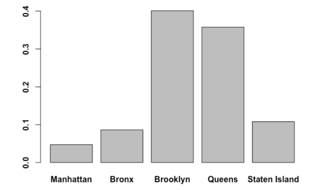
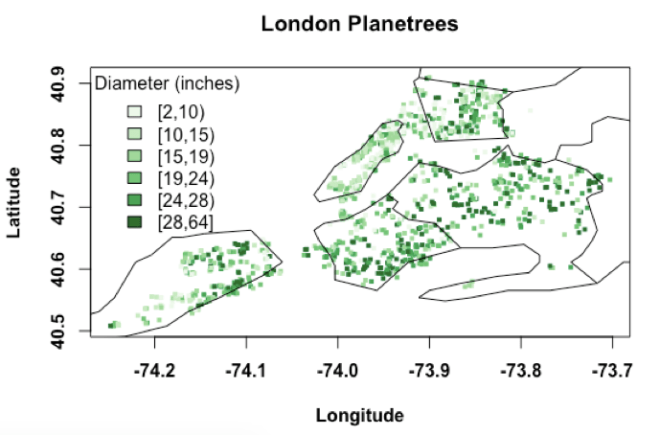
“Hmm 🙁 Let Manhattan at least have the old trees,” she prays and types the following lines to create a map of the trees and their diameters. She also wants to check where the damaged trees are.

There are some libraries required for making maps in R. If you don’t have them, you should install first using install.packages() command.

Jenny is plotting the diameter. plotvar.
The other lines are cosmetics, liners, lipsticks, and blush.

## Plot of London planetrees ##
 library(maps)
 library(maptools)
 library(RColorBrewer)
 library(classInt)
 library(gpclib)
 library(mapdata)
 library(fields)

 par(mfrow=c(1,2))
# plot 1: diameter
 plotvar <- lpt_true_distribution_diam
 
 nclr <- 6 # Define number of colours to be used in plot
 
 plotclr <- brewer.pal(nclr,"Greens") # Define colour palette to be used

# Define colour intervals and colour code variable for plotting
 class <- classIntervals(plotvar, nclr, style = "quantile")

 colcode <- findColours(class, plotclr)

 plot(lpt$longitude,lpt$Latitude,cex=0.15,pch=15, col = colcode, xlab="",ylab="",axes=F,font=2,font.lab=2)

 map("county",region="New York",add=T)
 box()

 title("London Planetrees")
 legend("topleft", legend = names(attr(colcode, "table")), fill = attr(colcode, "palette"), cex = 1, bty = "n",title="Diameter (inches)")

# plot 2: show damaged trees
 plotvar <- lpt_true_distribution_diam
 ind_1 = which(lpt$brnch_ligh=="Yes")

 nclr <- 6 # Define number of colours to be used in plot

 plotclr <- brewer.pal(nclr,"Greens") # Define colour palette to be used

# Define colour intervals and colour code variable for plotting
 class <- classIntervals(plotvar, nclr, style = "quantile")

 colcode <- findColours(class, plotclr)

 plot(lpt$longitude,lpt$Latitude,cex=0,pch=15, col = colcode, xlab="",ylab="",axes=F,font=2,font.lab=2)

 points(lpt$longitude[ind_1],lpt$Latitude[ind_1],pch=20,cex=0.1)

 map("county",region="New York",add=T)
 box()

 title("London Planetrees - Damaged")

The older trees belong mostly to Queens and Brooklyn; so do the damaged trees.

“This will make for a nice example of sampling bias, confidence intervals, and sampling strategies,” she thought as she noticed that the trees with smaller diameters are in Manhattan.

“If we only sample from Manhattan, it will clearly result in a bias in estimation of the population characteristics. Manhattan sample is not fully representative of the population or the true distribution,” she thought.

“Let me compare the population to the sample distributions from the five boroughs.”

She first separates the data for each borough and plots them against the true distribution.

## Breakdown by Borough
 lpt_manhattan = lpt[manhattan_index,]
 lpt_bronx = lpt[bronx_index,]
 lpt_brooklyn = lpt[brooklyn_index,]
 lpt_queens = lpt[queens_index,]
 lpt_staten = lpt[staten_index,]

# Plotting the population and borough wise samples ##
boxplot(lpt$tree_dbh,horizontal=T,xlim=c(0,7),ylim=c(-100,350),col="green",xlab="Diamter (inches)")

 boxplot(lpt_manhattan$tree_dbh,horizontal = T,add=T,at=2,col="red")
 text(-50,2,"Manhattan")

 boxplot(lpt_bronx$tree_dbh,horizontal = T,add=T,at=3,col="pink")
 text(-50,3,"Bronx")

 boxplot(lpt_brooklyn$tree_dbh,horizontal = T,add=T,at=4)
 text(-50,4,"Brooklyn")

 boxplot(lpt_queens$tree_dbh,horizontal = T,add=T,at=5)
 text(-50,5,"Queens")

 boxplot(lpt_staten$tree_dbh,horizontal = T,add=T,at=6)
 text(-60,6,"Staten Island")

 abline(v=lpt_true_mu,lty=2)
 text(30,0,"True Mean = 21.56 inches")

“Brooklyn, Queens and Staten Island resemble the population distribution. Manhattan and the Bronx are biased. If we want to understand the population characteristics, we need a random sample that covers all the five boroughs. The data seems to be stratified. Why don’t I sample data using different strategies and see how closely they represent the population,” she thought.

Simple Random Sampling

She starts with simple random sampling.

“I will use all five boroughs as my sampling frame. Each of these 87014 trees has an equal chance of being selected. Let me randomly select 30 trees from this frame using sampling without replacement. To show the variety, I will repeat this 10 times.”

She types up a few lines to execute this strategy.

# 1: Simple Random Sample
 population_index = 1:N

 ntimes = 10
 nsamples = 30

 simple_random_samples = matrix(NA,nrow=nsamples,ncol=ntimes)
 for (i in 1:ntimes)
 {
   # a random sample of 30 # 
   sample_index = sample(population_index,nsamples,replace=F)
   simple_random_samples[,i] = lpt$tree_dbh[sample_index]
 }

boxplot(lpt$tree_dbh,horizontal=T,xlim=c(0,11),ylim=c(-100,350),col="green",xlab="Diamter (inches)",main="Simple Random Sampling")

 boxplot(simple_random_samples,horizontal = T,boxwex=0.5,add=T,at=c(2:11),col="pink")

 abline(v=lpt_true_mu,lty=2,col="red")
 text(30,0,"True Mean = 21.56 inches")

The sampling is done ten times. These ten samples are shown in the pink boxes against the true distribution, the green box.

Most of the samples cover the true distribution. It is safe to say that the simple random sampling method is providing a reasonable representation of the population.

Stratified Random Sampling

“Let me now divide the population into strata or groups. I will have separate sampling frames for the five boroughs and will do a simple random sampling from each stratum. Since I know the percentages of the trees in each borough, I can roughly sample in that proportion and combine all the samples from the strata into a full representative sample. An inference from this combined samples is what has to be done, not on individual strata samples.”

# 2: Stratified Random Sample
 population_index = 1:N

 ntimes = 10
 nsamples = 100

 stratified_random_samples = matrix(NA,nrow=nsamples,ncol=ntimes)
 for (i in 1:ntimes)
 {
   # Manhattan # 
   ns_manhattan = round(nsamples*p_boro[1])   
   ns_bronx = round(nsamples*p_boro[2])
   ns_brooklyn = round(nsamples*p_boro[3])   
   ns_queens = round(nsamples*p_boro[4])
   ns_staten = nsamples - sum(ns_manhattan,ns_bronx,ns_brooklyn,ns_queens)
 
   sample_manhattan = sample(manhattan_index,ns_manhattan,replace=F)
   sample_bronx = sample(bronx_index,ns_bronx,replace=F)
   sample_brooklyn = sample(brooklyn_index,ns_brooklyn,replace=F)
   sample_queens = sample(queens_index,ns_queens,replace=F)
   sample_staten = sample(staten_index,ns_staten,replace=F)
 
   full_sample = c(lpt$tree_dbh[sample_manhattan],lpt$tree_dbh[sample_bronx],lpt$tree_dbh[sample_brooklyn],lpt$tree_dbh[sample_queens],lpt$tree_dbh[sample_staten])
   
   stratified_random_samples[,i] = full_sample
 }

boxplot(lpt$tree_dbh,horizontal=T,xlim=c(0,11),ylim=c(-100,350),col="green",xlab="Diamter (inches)",main="Stratified Random Sampling")

boxplot(stratified_random_samples,horizontal = T,boxwex=0.5,add=T,at=c(2:11),col="pink")

 abline(v=lpt_true_mu,lty=2,col="red")
 text(30,0,"True Mean = 21.56 inches")

Again, pretty good representation.

She was curious as to where Manhattan is in these samples. So she types a few lines to create this simple animation.

## Animation ##
 for (i in 1:10)
 {
 boxplot(lpt$tree_dbh,boxwex=0.3,horizontal=T,xlim=c(0,2),ylim=c(0,350),col="green",xlab="Diamter (inches)",main="Stratified Random Sampling")

   abline(v=lpt_true_mu,lty=2,col="red")
   text(50,0,"True Mean = 21.56 inches")
   legend(250,2,cex=0.76,pch=0,col="red","Manhattan")
   
stripchart(stratified_random_samples[6:100,i],add=T,at=1.5,cex=0.6,col="blue")

stripchart(stratified_random_samples[1:5,i],add=T,at=1.5,cex=0.75,col="red")

Sys.sleep(1)
 }

The animation is showing the samples each time. Manhattan samples are shown in red. Did you notice that the Manhattan samples are mostly from the left tail? Unless it is combined with the other strata, we will not get a full representative sample.

Cluster Random Sampling

“Both of these methods seem to give good representative samples. Let me now check the cluster random sampling method. We have the zip codes for each tree. So I will imagine that each zip code is a cluster and randomly select some zip codes using the simple random sampling method. All the trees in these zip codes will then be my sample.”

This is her code for the cluster sampling method. She first identifies all the zip codes and then randomly samples from them.

# 3: Cluster Random Sample
 zips = table(lpt$zipcode)
 list_zips = as.numeric(names(zips))
 list_zips = list_zips[-1]

 ntimes = 10
 nsamples = 10

 cluster_random_samples =  NULL
 for (i in 1:ntimes)
 {
   cluster_index = sample(list_zips,nsamples,replace=F)
   cluster_sample = NULL
   for (j in 1:length(cluster_index))
   {
     ind = which(lpt$zipcode==cluster_index[j])
     cluster_sample = c(cluster_sample,lpt$tree_dbh[ind])
   }
   cluster_random_samples = cbind(cluster_random_samples,cluster_sample)
 }
 boxplot(lpt$tree_dbh,horizontal=T,xlim=c(0,11),ylim=c(-100,350),col="green",xlab="Diamter (inches)",main="Cluster Random Sampling")

 boxplot(cluster_random_samples,horizontal = T,boxwex=0.5,add=T,at=c(2:11),col="pink",axes=F)

 abline(v=lpt_true_mu,lty=2,col="red")
 text(30,0,"True Mean = 21.56 inches")

“Hmm. There seems to be one sample which is biased. It is possible. We could have selected most of the zip codes from Manhattan or the Bronx. Since there is not much variability within these clusters, we could not represent the entire population. There is a risk of running poor inferences if we use this sample. Nevertheless, most times we get a good representative sample.”

Systematic Random Sampling

“Let me also try the systematic random sampling method just for completion. I will select every 870th tree in the line up of 87014 trees. I will do this 10 times moving one up, i.e., for the second try, I will select every 871st tree and so forth. Since I am covering the full range of the data, we should get a good representation.”

She types up a few simple lines.

# 4: Systematic Random Sample
 ntimes = 10
 nsamples = 100
 
systematic_random_samples = NULL
 for (i in 1:ntimes)
 {
   # a random sample of 30 # 
 systematic_index = seq(from = i, to = N, by = round((N/nsamples)))
 systematic_random_samples = cbind(systematic_random_samples,lpt$tree_dbh[systematic_index])
 }

boxplot(lpt$tree_dbh,horizontal=T,xlim=c(0,11),ylim=c(-100,350),col="green",xlab="Diamter (inches)",main="Systematic Random Sampling")

 boxplot(systematic_random_samples,horizontal = T,boxwex=0.5,add=T,at=c(2:11),col="pink",axes=F)

 abline(v=lpt_true_mu,lty=2,col="red")
 text(30,0,"True Mean = 21.56 inches")

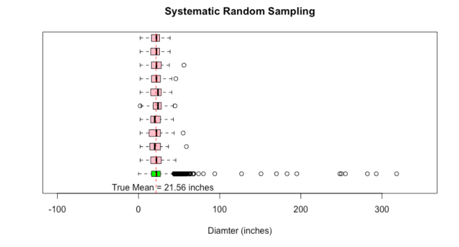
Things are good for this too.

“This dataset is an excellent resource to demonstrate so many concepts. I will use it to create a situational analysis for my class. I think I can show this over three weeks. Each week, I will introduce one concept. This Monday, I will take a small sample obtained from the simple random sampling method to the class. With this sample data, I will explain the basics of how to compute and visualize confidence intervals in R. I can also show how confidence intervals are derived using the bootstrap method.
Then, I will send them off on a task, asking them to collect data at random from the city. It will be fun hugging trees and collecting data. I should make sure I tell them that the data has to be collected at random from the entire City, not just a few boroughs. Then, all their samples will be representative, and I can show them the probabilistic interpretation of the confidence intervals, the real meaning.
After this, I will ask them to go out and take the samples again, only this time, I will emphasize that they should collect it from their respective boroughs. This means, the folks who collect data from Manhattan will bring biased samples and they will easily fall out in the confidence interval test. This will confuse them !! but it will give a good platform to explain sampling bias and the various strategies of sampling.”

Someday, I shall be gone; yet, for the little I had to say, the world might bear, forever its tone.

If you find this useful, please like, share and subscribe.
You can also follow me on Twitter @realDevineni for updates on new lessons.

Lesson 82 – Riding with confidence, in R: Week 3

On the eleventh day of February 2019, Jenny showed her students how to compute and visualize confidence intervals in R. Her demo included the confidence interval on the mean, variance/standard deviation, and proportions. She also presented the code to develop bootstrap confidence intervals for any parameter. All this was based on a random sample that she collected.

But she wanted the students to have hands-on experience of data gathering and know the real meaning of confidence intervals, in that, for a 95% level, there is a 95% probability of selecting a sample for which the confidence interval will contain the true parameter value, $\mu, \sigma^{2}$ or p. So she sent them out to collect data through random sampling. The 40 students each brought back samples. 40 different samples of 30 trees each.

~~~~~~~~~~~~~~~~~~~~~~~~~~~~~~~~~~~~~~~~~~~~~~~~~~~~~~~~~~~~~~

On the eighteenth day of February 2019, the students came back with the samples. They all developed confidence intervals from their samples. Jenny showed them how the sample mean was converging to the true mean, and that over 40 confidence intervals, roughly two (5%) may not contain the truth. They also learned how the interval shrinks as one gets more and more samples.

Then, Jenny wanted them to understand the issues with sampling. So she sent them off for a second time. This time, the students divided themselves into teams, visiting different boroughs and collecting samples only from that borough.

Today, they are all back with their new samples.

~~~~~~~~~~~~~~~~~~~~~~~~~~~~~~~~~~~~~~~~~~~~~~~~~~~~~~~~~~~~~~

Monday, February 25, 2019

In which the students come back with new samples, borough wise. Jenny explains the traps due to sampling bias and the basic types of sampling strategies.

It is Samantha who is always at the forefront of the class. She was leading seven other students in team Manhattan. Each of these eight students gathered data for 30 trees in Manhattan. So, they create eight different confidence intervals — representing the intervals from Manhattan. Samantha shows her example — the locations of the data that she gathered and the confidence interval of the true mean.

The 95% confidence interval of the true mean diameter $\mu$ is $\bar{x} - t_{0.025,(n-1)}\frac{s}{\sqrt{n}} \le \mu \le \bar{x} + t_{0.025,(n-1)} \frac{s}{\sqrt{n}}$

“This sample may or may not contain the true mean diameter, but I know that there is a 95% probability of selecting this sample which when used to develop the confidence intervals, will contain the truth,” she said.

John was heading team Bronx. He followed Samantha to show the places he visited and the confidence interval from his sample. His team also had eight students, and each of them gathered data for 30 trees from the Bronx.

John strongly feels that he may be the unfortunate one whose confidence interval will not contain the truth. He may be one among the two. Let’s see.

The leaders of the other three teams, Justin, Harry, and Susan also prepare their confidence intervals. They all go up to the board and display their intervals.

“From last week, we know that the approximation for the true mean $\mu$ is 21.3575,” said Samantha as she projects the vertical line to show it. As you all know, Jenny showed last week that the sample mean was converging to 21.3575 as the samples increased. The principle of consistency.

As they discuss among themselves, Jenny entered the room and gazed at the display. She knew something that the students did not know. But she concealed her amusement and passed along the file to collect the data from all 40 students.

Like last week, the students fill out the file with the data they collected, borough wise. The file will have a total of 1200 row entries. Here is the file. As you have rightly observed, the boro code column is now ordered since the file went from team Manhattan to team Staten Island.

Jenny used the same lines as last week to create a plot to display all the 40 confidence intervals.

Assuming that the file is in the same folder you set your working directory to, you can use this line to read the data into R workspace.

# Reading the tree data file from the students - boro wise #
students_data_boro = read.csv("students_data_borough.csv",header=T)

Use these lines to plot all the confidence intervals.

# Jenny puts it all together and shows #
# 40 students went to collect data from specific boroughs in NYC #
# Each student collects 30 samples #
# Each student develops the confidence intervals #
 
 nstudents = 40
 nsamples = 30
 
 students = 1:nstudents

 alpha = 0.95
 t = alpha + (1-alpha)/2
 
 sample_mean = matrix(NA,nrow=nstudents,ncol=1)
 sample_sd = matrix(NA,nrow=nstudents,ncol=1)
 ci_t = matrix(NA,nrow=nstudents,ncol=2)
 
 for(i in 1:nstudents)
 {
   ind = which(students_data_boro$student_index == i)
 sample_data = students_data_boro$tree_dbh[ind]
 sample_mean[i] = mean(sample_data)
 sample_sd[i] = sd(sample_data)
 cit_lb = sample_mean[i] - qt(t,df=(n-1))((sample_sd[i]/sqrt(n)))   
 cit_ub = sample_mean[i] + qt(t,df=(n-1))((sample_sd[i]/sqrt(n)))
 ci_t[i,] = c(cit_lb,cit_ub)
 }

# Plot all the CIs #
 stripchart(ci_t[1,],type="l",col="green",main="",xlab="Diameter (inches)",xlim=c(9,30),ylim=c(1,nstudents))
 
 stripchart(sample_mean[1],add=T,col="green")

 for (i in 2:nstudents)
 {
   stripchart(ci_t[i,],type="l",col="green",main="",add=T,at = i)
   stripchart(sample_mean[i],col="green", add=T, at = i)
 }

Once you execute these lines, you will also see this plot in your plot space.

“It looks somewhat different than the one we got last time,” said John.
“Let me see how many of them will contain the truth,” he added as he typed these lines.

He looks through all the confidence intervals for whether or not they cover the truth using an if statement. He calls them “false_samples.” Then, he plots all the confidence intervals once again, but this time, he uses a red color for the false samples. He also added the borough names to give a reference point.

nyc_random_truth = 21.3575

false_samples = students

 for (i in 1:nstudents)
 {
   if( (ci_t[i,1] > nyc_random_truth) || (ci_t[i,2] < nyc_random_truth) ) 
 {false_samples[i]=1} else 
 {false_samples[i]=0}
 }

false_ind = which(false_samples == 1)

# Plot all the CIs; now show the false samples #
 stripchart(ci_t[1,],type="l",col="green",main="",xlab="Diameter (inches)",xlim=c(9,30),ylim=c(1,nstudents))

 stripchart(sample_mean[1],add=T,col="green")

 for (i in 2:nstudents)
 {
   stripchart(ci_t[i,],type="l",col="green",main="",add=T,at = i)
   stripchart(sample_mean[i],add=T,col="green",at = i)
 }

 abline(v=nyc_random_truth,lwd=3)

 for (i in 1:length(false_ind))
 {
   j = false_ind[i]
 stripchart(ci_t[j,],type="l",col="red",lwd=3, main="", add = T, at = j)
   stripchart(sample_mean[j],col="red", lwd=3, add=T, at = j)
 }

 text(18,4,"Manhattan")
 text(24,12,"Bronx")
 text(27,20,"Brooklyn")
 text(28,28,"Queens")
 text(28,37,"Staten Island")

Try it yourself. You will also see this plot.

The students are puzzled. Clearly, there are more than 5% intervals that do not cover the truth. Why?

Jenny explains sampling bias

Jenny now explains to them about sampling bias. She starts with a map of all the data that the students brought.

We will get a more detailed explanation for creating maps in R in some later lessons. For now, you can type these lines that Jenny used to create a map.

### Full Map ###
 library(maps)
 library(maptools)
 library(RColorBrewer)
 library(classInt)
 library(gpclib)
 library(mapdata)
 library(fields)
 
 plotvar <- students_data_boro$tree_dbh
 
 nclr <- 6 # Define number of colours to be used in plot
 
 plotclr <- brewer.pal(nclr,"Greens") # Define colour palette to be used
 
# Define colour intervals and colour code variable for plotting
 class <- classIntervals(plotvar, nclr, style = "quantile")
 colcode <- findColours(class, plotclr)
 plot(students_data_boro$longitude,students_data_boro$Latitude,cex=0.55,pch=15, col = colcode, xlab="Longitude",ylab="Latitude",font=2,font.lab=2)

 map("county",regions ="New York",add=T)

 title("London Planetrees")

 legend("topleft", legend = names(attr(colcode, "table")), fill = attr(colcode, "palette"), cex = 1, bty = "n",title="Diameter (inches)")

“Look at this map. I am showing the location of the tree based on the latitude and longitude you all recorded. Then, for each point, I am also showing the diameter of the tree using a color bar. Thick trees, i.e., those with larger diameters are shown in darker green. Likewise, thin trees are shown in lighter green. Do you notice anything?” asked Jenny.

Samantha noticed it right away. “The trees in Manhattan have smaller diameters. Mostly, they have dull green shade,” she said.

“Precisely,” Jenny continues. “The trees are not all randomly distributed. They are somewhat clustered with smaller diameters in Manhattan and Bronx and larger diameters in the other boroughs.

Since you collected all your samples from a specific borough, there is a risk of sampling bias.

We can make good inferences about the population only if the sample is representative of the population as a whole.

In other words, the distribution of the sample must be like the distribution of the population from which it comes. In our case, the trees in Manhattan are not fully representative of the entire trees in the City. There was sampling bias, a tendency to collect a sample that is not entirely representative of the population.

For team Manhattan, since the distribution of your sample is dissimilar to that of the population, your statements about the truth are not accurate. You will have a bias — poor inference.

See, the sample mean also does not converge. Even at n=1200, there is still some element of variability.

Last week when you collected data for the trees, I asked you to gather them randomly by making sure that you visit all the boroughs. In other words, I asked you to collect random samples. Randomly visiting all the boroughs will avoid the issues arising from sampling bias. They give a more representative sample and minimize the errors in the inference. That is why we did not see this bias last week.”

“Are there types of sampling?” asked Justin.

Jenny replied. “At the very basic level, “simple random sampling” method, “stratified random sampling” method and “cluster random sampling” method. One of these days, I will show you how to implement these sampling strategies in R. For now let’s talk about their basics.

What you did in the first week was a simple random sampling method. Your sampling frame was all possible London planetrees in NYC. Each tree in this frame has an equal chance of being selected. From this frame, you randomly selected 30 trees. This is sampling without replacement. You did not take the measurements for the same tree two times. Computationally, what you did was to draw without replacement, a sequence of n random numbers from 1 to N. Mostly, you will get an equal proportion of trees from each borough.

Then there is the stratified random sampling method. Here, we can divide the population into strata — subpopulations or separate sampling frames. Within each frame or strata, we can do simple random sampling to collect data. The number of samples taken from each stratum or subpopulation is proportional to the size of the stratum. In other words, if we know the percent number of trees in Manhattan compared to the total number of trees, we can approximately sample that percentage from the Manhattan strata. One thing I can do is to assume that each of your teams got a simple random sample from a stratum, and combine the five teams to give me a full representative sample. An inference from this combined sampled will be more accurate than individual strata samples.

In the cluster random sampling method, we can first divide the population into clusters and then randomly select some clusters. The data from these clusters will make up the sample. Imagine that we divide the city into zip codes — each zip code is a cluster. Then we can randomly select some zip codes as part of our sampling strategy. All the trees in these zip codes make up our cluster random sample. However, if there is not much variability within each cluster, we run the risk of not representing the entire population, and hence poor inference.

We can also do systematic sampling, like selecting every 10th tree, but again, we should ensure that we cover the range. If not, we might get a biased sample.”

“How did you know that the borough wise sampling would be biased?” asked someone.

Well, for a one-line answer, you can say it was an educated guess. For a one-lesson answer, you should wait till next week.

If you find this useful, please like, share and subscribe.
You can also follow me on Twitter @realDevineni for updates on new lessons.

Lesson 81 – Riding with confidence, in R: Week 2

Monday, February 18, 2019

In which the students come back with samples. Jenny shows them sampling distributions, the real meaning of confidence interval, and a few other exciting things using their data. She sends them off on a second task.

Where is the Mean

Samantha, John, and Christina explore

Samantha: These are the London planetrees I have data for.

The $100(1-\alpha)\%$ confidence interval of the population mean ( $\mu$ ) is the interval $[\bar{x} - t_{\frac{\alpha}{2},(n-1)}\frac{s}{\sqrt{n}}, \bar{x} + t_{\frac{\alpha}{2},(n-1)} \frac{s}{\sqrt{n}}]$ .

I have a sample of 30 trees. For these 30 trees, the sample mean is 20.6 inches and the sample standard deviation is 9.06 inches. Based on this, the confidence interval of $\mu$ is $[20.6 - 2.05\frac{9.06}{\sqrt{30}}, 20.6 + 2.05\frac{9.06}{\sqrt{30}}]$ .

[17.22 inches, 23.98 inches]

John: I collected data for 30 trees too. Here is my data.

And here is the confidence interval I came up with; [17.68 inches, 24.05 inches]. For my data, the sample mean is 20.87 inches and the sample standard deviation is 8.52 inches.

Christina: I have a sample of 30 too. Here is where I took them from.

And, here is the 95% confidence interval of the mean; [19.9 inches, 24.9 inches].

Their sample statistics are different. Their confidence intervals are different. They begin to wonder whether their interval contains the truth, $\mu$ , or, whose interval contains the truth?

Jenny puts all the intervals in context

Jenny shares with the students, an empty data file with the following headers.

The students fill out the file with the data they collected last week. Her class has 40 students, so when the file came back to Jenny, it had a total of 40*30 = 1200 row entries.

Jenny uploaded this file here, for the analysis she is going to show the class.

Jenny: I am sure you all had much fun last week visiting different places in the city and collecting data for the analysis. I am hoping that all of you randomly selected the places to visit. Based on what Sam and Christina showed, it looks like the places are fairly spread out — so we would have gotten a random sample from the population of the trees.

Sam, John, and Christina; the three of them computed the 95% confidence interval of the true mean $\mu$ based on their sample statistics. They found their intervals to be different.

Let’s look at all the 40 confidence intervals. Now that I have the data from you all, I will show you how to do it in R. Essentially, I will take each one of your data, compute the sample statistics and use them to compute the respective confidence intervals. We have 40 different samples, so we will get 40 different confidence intervals — each interval is a statement about the truth. If you remember what we have been discussing about the confidence intervals, for a 95% confidence level,

There is a 95% probability of selecting a sample whose confidence interval will contain the true value of $\mu$ .

In other words, approximately 95% of the 40 samples (38 of them) may contain the truth. 5% (2 of them) may not contain the truth.

Let’s see who is covering the truth and who is not!

I want you all to work out the code with me. Here we go.

First, we will read the data file into R workspace.

# Reading the tree data file from the students # 
 students_data = read.csv("students_data.csv",header=T)

Next, use the following lines to compute the confidence interval for each student. I am essentially repeating the computation of sample mean, sample standard deviation and the confidence intervals, in a loop, 40 times, one for each student.

#40 students went to collect data from random locations in NYC # 
#Each student collects 30 samples #
#Each student develops the confidence intervals #
 
 nstudents = 40
 nsamples = 30
 
 students = 1:nstudents

 alpha = 0.95
 t = alpha + (1-alpha)/2
 
 sample_mean = matrix(NA,nrow=nstudents,ncol=1)
 sample_sd = matrix(NA,nrow=nstudents,ncol=1)
 
 ci_t = matrix(NA,nrow=nstudents,ncol=2)
 
 for(i in 1:nstudents)
  {
  ind = which(students_data$student_index == i)
  
  sample_data = students_data$tree_dbh[ind]
  
  sample_mean[i] = mean(sample_data)
  sample_sd[i] = sd(sample_data)
  
  cit_lb = sample_mean[i] - qt(t,df=(n-1))((sample_sd[i]/sqrt(n)))   
  cit_ub = sample_mean[i] + qt(t,df=(n-1))((sample_sd[i]/sqrt(n)))
  
  ci_t[i,] = c(cit_lb,cit_ub)
  }

Now, let’s plot the 40 intervals to see them better. A picture is worth a thousand numbers. Use these lines. They explain themselves.

#Plot all the CIs #
stripchart(ci_t[1,],type="l",col="green",main="",xlab="Diameter (inches)",xlim=c(15,30),ylim=c(1,nstudents))
stripchart(sample_mean[1],add=T,col="green")

for (i in 2:nstudents)
 {
   stripchart(ci_t[i,],type="l",col="green",main="",add=T,at = i)
   stripchart(sample_mean[i],col="green", add=T, at = i)
 }

The students are overjoyed looking at the pretty image.

John: This is neat. All our intervals are different, owing to each one of us bringing a different random sample. How we know which one of us contains the truth and which one of us does not is still not clear.

Jenny: We can get a close approximation based on the principle of consistency.

$\displaystyle{\lim_{n\to\infty} P(|T_{n}(\theta)-\theta|>\epsilon)} \to 0$

As n approaches infinity, the sample estimate approaches the true parameter. We can take the full data record that you all brought, 1200 data points and compute the overall mean.

true_mu = mean(students_data$tree_dbh)

While it is not exactly the true value, based on the idea of consistency, we can assume that it is converging to the true one.

$\mu$ = 21.3575 inches.

Look at this.

# Truth Convergence Plot #
 true_mean = sample_mean
 for (i in 1:nstudents)
 {
   ind = which(students_data$student_index <= i)
   true_mean[i] = mean(students_data$tree_dbh[ind])
 }

plot(true_mean,type="o",xlab="Increasing Sample",ylab="Convergence of the Sample Mean",font=2,font.lab=2,ylim=c(20,22))

My sixth sense and divine visions also tell me that this is converging to the truth!

Now, we can check which of these intervals contains the true mean $\mu$ , 21.3575 inches.

You can use this simple code to check.

false_samples = students
 for (i in 1:nstudents)
 {
   if( (ci_t[i,1] > true_mu) || (ci_t[i,2] < true_mu) ) 
 {false_samples[i]=1} else    
  {false_samples[i]=0}
 }
 false_ind = which(false_samples == 1)

It looks like number 4 and number 26 are not covering the truth. Harry and Miguel.

Let us point them out. Here, look at another pretty plot. The thick black vertical line is the truth, 21.3575 inches. The brown line is how the sample mean ( $\bar{x}$ ) is converging to the truth ( $\mu$ ) as we collect more samples. Harry and Miguel stand out. That is 2 out of 40; 5%.

# Plot all the CIs; now show the false samples #
 stripchart(ci_t[1,],type="l",col="green",main="",xlab="Diameter (inches)",xlim=c(15,30),ylim=c(1,nstudents))
 stripchart(sample_mean[1],add=T,col="green")
 
for (i in 2:nstudents)
 {
   stripchart(ci_t[i,],type="l",col="green",main="",add=T,at = i)
   stripchart(sample_mean[i],add=T,col="green",at = i)
 }

 abline(v=true_mu,lwd=3)
 lines(true_mean,students,type="o",col="brown",cex=0.5)

 for (i in 1:length(false_ind))
 {
   j = false_ind[i]

 stripchart(ci_t[j,],type="l",col="red",lwd=3, main="", add = T, at = j)
   stripchart(sample_mean[j],col="red", lwd=3, add=T, at = j)
 }

 text(16,4.6,"Harry")
 text(26,26.6,"Miguel")

There is a 95% probability of selecting a sample whose confidence interval will contain the true value of $\mu$ .

Miguel: What happens to the confidence interval when we compute it with larger sample sizes? I mean, what is the relationship between the confidence interval and sample size?

Jenny: Look at the equation for the confidence interval of the population mean; $[\bar{x} - t_{\frac{\alpha}{2},(n-1)}\frac{s}{\sqrt{n}}, \bar{x} + t_{\frac{\alpha}{2},(n-1)} \frac{s}{\sqrt{n}}]$ .

Theoretically, as n tends to infinity, the interval shrinks to 0 since the sample mean converges to the true mean. So, as n gets larger, the interval gets smaller. Let me show you how it works. Take our data, and, just as we computed the sample mean for increasing sample size to see the convergence, compute the confidence interval also at each step.

# How does CI change with more sample size
 sample_mean_update = matrix(NA,nrow=nstudents,ncol=1)
 sample_sd_update = matrix(NA,nrow=nstudents,ncol=1)
 
ci_t_update = matrix(NA,nrow=nstudents,ncol=2)

 for(i in 1:nstudents)
 {
 ind = which(students_data$student_index <= i)
 ns = length(ind)

 sample_data = students_data$tree_dbh[ind]

 sample_mean_update[i] = mean(sample_data)
 sample_sd_update[i] = sd(sample_data)

cit_lb = sample_mean_update[i] - qt(t,df=(ns-1))((sample_sd_update[i]/sqrt(ns)))   
cit_ub = sample_mean_update[i] + qt(t,df=(ns-1))((sample_sd_update[i]/sqrt(ns)))
 
ci_t_update[i,] = c(cit_lb,cit_ub)
 }

Now, we can plot these confidence intervals against increasing sample size to see what happens. Just remember that each interval is an interval that is based on an increased sample size than the previous. The first interval has 30 data points, the second one has 60 data points, the third one, 90, the fourth, 120 etc.

# Plot all the CIs #
 stripchart(ci_t_update[1,],vertical=T,type="l",col="green",main="",ylab="Diameter (inches)",ylim=c(16,25),xlim=c(1,nstudents),xlab="Increasing Sample Size")
stripchart(sample_mean_update[1],vertical=T,add=T,col="green")

 for (i in 2:nstudents)
 {
   stripchart(ci_t_update[i,],type="l",col="green",main="",add=T,at = i,vertical=T)
   stripchart(sample_mean_update[i],col="green", add=T, at = i,vertical=T)
 }
 
lines(students,true_mean,type="o",col="brown",cex=0.5)

See how the interval gets smaller and smaller as the sample size increases. If we do this enough number of times, the interval vanishes — as we will approach the entire population.

T or Z

Christina: If we have a large sample, why can’t we use $[\bar{x} - Z_{\frac{\alpha}{2}}\frac{\sigma}{\sqrt{n}} \le \mu \le \bar{x} + Z_{\frac{\alpha}{2}}\frac{\sigma}{\sqrt{n}}]$ as the $100(1-\alpha)\%$ confidence interval for the true mean $\mu$ ? For a large sample size, we can assume s, the sample standard deviation of the large sample as $\sigma$ .

Jenny: Yes, we can do that. As n increases, the difference between T and Z is minimal. However, it is better to use t-distribution for confidence intervals of $\mu$ , so we don’t fall into traps. I will show those traps next week.

Where is the Standard Deviation and Proportion

Jenny: Can you follow the same logic and develop the confidence intervals for $\sigma$ ? How many of you will cover the truth, how many of you will not?

Again, approximately, 95% of the intervals will cover the true $\sigma$ , i.e., roughly 38 of your intervals will have the truth, 2 will not. Check this out.

alpha = 0.95
u = alpha + (1-alpha)/2
l = 1 - u
 
sample_var = matrix(NA,nrow=nstudents,ncol=1)
ci_sd = matrix(NA,nrow=nstudents,ncol=2)

 for(i in 1:nstudents)
 {
  ind = which(students_data$student_index == i)
  ns = length(ind)
 
  sample_data = students_data$tree_dbh[ind]

  sample_var[i] = var(sample_data)

  chi_low = ((ns-1)sample_var[i])/qchisq(u,df=(ns-1))   
  chi_up = ((ns-1)sample_var[i])/qchisq(l,df=(ns-1))

  ci_sd[i,] = c(sqrt(chi_low),sqrt(chi_up))
 }

true_sd = sqrt((sum((students_data$tree_dbh-true_mu)^2))/length(students_data$tree_dbh))

# False samples #
false_samples_sd = students
 for (i in 1:nstudents)
 {
   if( (ci_sd[i,1] > true_sd) || (ci_sd[i,2] < true_sd) ) 
 {false_samples_sd[i]=1} else 
 {false_samples_sd[i]=0}
 }

false_sd_ind = which(false_samples_sd == 1)

# Plot all the CIs; now show the false samples #
stripchart(ci_sd[1,],type="l",col="green",main="CI on Standard Deviation",xlab="Diameter (inches)",xlim=c(5,15),ylim=c(1,nstudents))
stripchart(sample_sd[1],add=T,col="green")
 
for (i in 2:nstudents)
 {
   stripchart(ci_sd[i,],type="l",col="green",main="",add=T,at = i)
   stripchart(sample_sd[i],add=T,col="green",at = i)
 }
 
abline(v=true_sd,lwd=3)

Jenny: Here all the intervals cover the truth, but, in the long-run, 95% of the intervals cover the truth.

John: How about proportion?

Jenny: Yes, can you all develop the confidence intervals for the proportion of damaged trees? I want you to use bootstrap confidence intervals for p instead of the one based on the assumption of normal distribution.

So the students typed away a few lines of code to finally create this.

# Confidence Interval of p #
 alpha = 0.95
 u = alpha + (1-alpha)/2
 l = 1 - u
 
nboot = 1000

 sample_p = matrix(NA,nrow=nstudents,ncol=1)
 ci_p_boot = matrix(NA,nrow=nstudents,ncol=2)

 for(i in 1:nstudents)
 {
   ind = which(students_data$student_index == i)
 ns = length(ind)

 sample_data = students_data$brnch_ligh[ind]

 sample_p[i] = length(which(sample_data=="Yes"))/ns

 bootstrap_replicate_proportion = matrix(NA,nrow=nboot,ncol=1)
 for (j in 1:nboot)
     {
       ind2 = 1:ns
   bootstrap_ind = sample(ind2,ns,replace=T)   
bootstrap_sample_damage = sample_data[bootstrap_ind]   
bootstrap_replicate_proportion[j,1] = length(which(bootstrap_sample_damage=="Yes"))/ns }
 
ci_p_boot[i,] = quantile(bootstrap_replicate_proportion,c(l,u))
 }
 
true_p = length(which(students_data$brnch_ligh=="Yes"))/length(students_data$brnch_ligh)

# False samples #
 false_samples_p = students
 for (i in 1:nstudents)
 {
   if( (ci_p_boot[i,1] > true_p) || (ci_p_boot[i,2] < true_p) ) 
 {false_samples_p[i]=1} else 
 {false_samples_p[i]=0}
 }
 
false_p_ind = which(false_samples_p == 1)

# Plot all the CIs; now show the false samples #
 stripchart(ci_p_boot[1,],type="l",col="green",main="CI on Proportion",xlab="Proportion",xlim=c(0,0.5),ylim=c(1,nstudents))
 stripchart(sample_p[1],add=T,col="green")

 for (i in 2:nstudents)
 {
   stripchart(ci_p_boot[i,],type="l",col="green",main="",add=T,at = i)
   stripchart(sample_p[i],add=T,col="green",at = i)
 }

 abline(v=true_p,lwd=3)

 for (i in 1:length(false_p_ind))
 {
   j = false_p_ind[i]
 stripchart(ci_p_boot[j,],type="l",col="red",lwd=3, main="", add = T, at = j)
   stripchart(sample_p[j],col="red", lwd=3, add=T, at = j)
 }

You can also check out their full code here.

As the class comes to an end, Samantha looks fulfilled. “Wow, that is quite a day,” she said. “We covered many things today, but more importantly the true meaning of the confidence intervals. There is a 95% probability of selecting a sample whose confidence interval will contain the true value.”

“Assuming our data is collected without any bias,” interjected Jenny. The students looked puzzled.

“This week, I want you to go out and collect the data again, but this time, divide yourselves into boroughs. Eight of you will belong to team Manhattan and will collect tree data from Manhattan only. You will still collect data randomly but will do it only from Manhattan. Eight of you are team Queens and you collect data randomly from Queens. The other three teams, team Bronx, team Brooklyn, and team Staten Island will do the same in their boroughs. We will again have 30 trees each, and a total of 1200 trees.”

So, the students go off on another mission. Some of them are still puzzled or rather have a “what difference does it make” face on them. Some of them are as usual excited to hug the trees again. We will all wait and see what they come up with. More fun with data.

If you find this useful, please like, share and subscribe.
You can also follow me on Twitter @realDevineni for updates on new lessons.

Lesson 80 – Riding with confidence, in R: Week 1

Monday, February 11, 2019

In which Jenny shows her students how to compute and visualize confidence intervals in R, and sends them off on a task.

“Did you know that the symbol of the department of parks and recreations is a cross between the leaf of the London plane and a maple leaf?” asked Jenny as she opened her high school data class. She volunteered to help 40 high school kids recently.

The obvious response from the kids is no response.

“It is,” she said. “More than 10% of the trees are London Planetrees. They grow up to 20 – 30 meters, with a trunk circumference of 3 meters.”

She projected a map on the big screen.

“These are the places I randomly selected to visit and record the diameter of the trunk of the London planetrees. You have this data in the handout. We will learn how to develop confidence intervals in R.”

For your analysis in R, the data file can be downloaded from here.”

Let’s Start with the Mean

“Can someone tell me how we can get the confidence interval of the mean diameter?” she asked.

John raised his hand to answer. “Yes, John, go ahead,” said Jenny.

“The $100(1-\alpha)\%$ confidence interval for the true mean $\mu$ is $[\bar{x} - Z_{\frac{\alpha}{2}}\frac{\sigma}{\sqrt{n}} \le \mu \le \bar{x} + Z_{\frac{\alpha}{2}}\frac{\sigma}{\sqrt{n}}]$ . If the sample size n is very large, we can substitute the sample standard deviation s in place of the unknown $\sigma$ . However, for small sample sizes, the sample standard deviation s is itself subject to error. It may be far from the true value of $\sigma$ . So it is preferable to use t-distribution for the confidence interval of the mean since $\frac{\bar{x}-\mu}{\frac{s}{\sqrt{n}}}$ tends to a t-distribution with (n-1) degrees of freedom.

So I would say that the $100(1-\alpha)\%$ confidence interval of the population mean is the interval $[\bar{x} - t_{\frac{\alpha}{2},(n-1)}\frac{s}{\sqrt{n}}, \bar{x} + t_{\frac{\alpha}{2},(n-1)} \frac{s}{\sqrt{n}}]$ .”

“Excellent. Let’s all compute the 95% confidence interval of the mean diameter of the trunk of the London planetrees from the sample I gave you. The 95% confidence interval of the true mean diameter ( $\mu$ ) is $\bar{x} - t_{0.025,(n-1)}\frac{s}{\sqrt{n}} \le \mu \le \bar{x} + t_{0.025,(n-1)} \frac{s}{\sqrt{n}}$ .”

They all started calculating. Some of them pulled out t-tables to get the t-critical ( $t_{0.025,29}$ ), i.e., the quantile from the t-distribution corresponding to the upper tail probability of 0.025, and 29 degrees of freedom.

Jenny stopped them. “Don’t compute the interval by hand. Let’s do it in R.”

“Read the data file first. I am assuming that you all have the file in the same folder that you set the working directory to.”

# Read the data file -- Jenny's sample data #
jenny_sample_data = read.csv("jenny_data.csv",header=T)
nsamples = nrow(jenny_sample_data)

“Did you notice that the file has seven columns? The diameter of the tree trunk is recorded in the first column, tree_dbh. I am sure you figured out what the other columns are, except maybe the column that reads brnch_ligh that has Yes or No as the inputs. We will get to that in a bit.”

“Let’s compute the sample mean ( $\bar{x}$ ), sample variance ( $s^{2}$ ), and the sample standard deviation ( $s$ ).”

#statistics of the sample #
jenny_samplemu = mean(jenny_sample_data$tree_dbh)
jenny_samplevar = var(jenny_sample_data$tree_dbh)
jenny_samplesd = sd(jenny_sample_data$tree_dbh)

“What you were about to look up from the t-table can be obtained using this command in R.”

qt(0.975,df=29)

[1] 2.04523

“The t-critical value is 2.04523.”

“We can write a few lines to compute the confidence interval for any $\alpha$ level, and show them graphically.”

# Confidence interval of the mean using t-distribution #
alpha = 0.95 # 95% confidence interval 
t = alpha + (1-alpha)/2
n = nsamples

cit_lb = jenny_samplemu - qt(t,df=(n-1))*((jenny_samplesd/sqrt(n))) 
cit_ub = jenny_samplemu + qt(t,df=(n-1))*((jenny_samplesd/sqrt(n)))

ci_t = c(cit_lb,cit_ub)

stripchart(ci_t,type="l",lwd=3,col="green",main="CI on Mean",xlab="Diameter (inches)")
stripchart(jenny_samplemu,add=T,lwd=3,col="green")

“The sample mean ( $\bar{x}$ ) is 22.433 inches and the intervals extend out to 19.67 inches on the left and 25.20 inches on the right.”

“There is a 95% probability of selecting this sample for which the confidence interval will contain the true value of $\mu$ .”

The kids looked happy seeing the image on their screen.

Next, let’s explore the Variance and the Standard Deviation

“Do you remember the equation for the confidence interval of the variance and the standard deviation?” Jenny asked.

Samantha wanted to answer.

“The $100(1-\alpha)\%$ confidence interval of the population variance $\sigma^{2}$ is the interval $[\frac{(n-1)s^{2}}{\chi_{u,n-1}}, \frac{(n-1)s^{2}}{\chi_{l,n-1}}]$ . We can get the square roots of the confidence limits to get the confidence interval on the true standard deviation,” she said.

“The interval $[\sqrt{\frac{(n-1)s^{2}}{\chi_{u,n-1}}}, \sqrt{\frac{(n-1)s^{2}}{\chi_{l,n-1}}}]$ is called the $100(1-\alpha)\%$ confidence interval of the population standard deviation $\sigma$ .”

Jenny was pleased. She has an outstanding cohort. They always come prepared.

“Yes. In our case, $\frac{(n-1)s^{2}}{\sigma^{2}}$ follows a Chi-square distribution with 29 degrees of freedom. The lower and upper critical values at the 95% confidence interval $\chi_{l,29}$ and $\chi_{u,29}$ can be obtained from the Chi-square table, or, as you guessed, can be computed in R using a simple command. Try these,” she said.

qchisq(0.975,df=29)

[1] 45.72229

qchisq(0.025,df=29)

[1] 16.04707

“Of course, we can automate this and make nice graphics for the intervals. Use this code.”

# Confidence interval of the variance and standard deviation using Chisq-distribution #
u = alpha + (1-alpha)/2
l = 1 - u

chi_low = ((n-1)*jenny_samplevar)/qchisq(u,df=(n-1)) 
chi_up = ((n-1)*jenny_samplevar)/qchisq(l,df=(n-1))

ci_var = c(chi_low,chi_up)
ci_sd = c(sqrt(chi_low),sqrt(chi_up))

stripchart(ci_var,type="l",lwd=3,col="green",main="CI on Variance",xlab="Diameter^2 (inches^2)")
stripchart(jenny_samplevar,add=T,lwd=3,col="green")

stripchart(ci_sd,type="l",lwd=3,col="green",main="CI on Standard Deviation",xlab="Diameter (inches)")
stripchart(jenny_samplesd,add=T,lwd=3,col="green")

“The sample variance is 54.74 $inches^{2}$ , with a lower bound of 34.72 $inches^{2}$ and an upper bound of 98.92 $inches^{2}$ . Notice how the intervals are not symmetric. Do you remember why?”

“The sample standard deviation is 7.40 inches. The 95% lower and upper bounds are 5.90, and 9.95 inches respectively.”

The kids spent a few minutes typing up the lines of code to get the intervals and make the graphics.

Jenny continued the lesson.

“Now, look at the third column in the data file, brnch_ligh. When I measured the trunk circumference, I also noticed that, for some trees, there were branch problems caused by lights or wires. I recorded this as a “yes” or a “no” depending on whether or not there was a problem. Who would think to have nice colorful lights on the trees would be damaging 🙁

Can one of you count through the sample and tell me what is the estimate of the proportion of trees ( $\hat{p}$ ) that are damaged.”

“0.1,” someone answered from the back.

“Great, now, that invisible person, can you tell me how we can compute the confidence interval of the true proportion?”

Christina it was. She answered, “the $100(1-\alpha)%$ confidence interval for the true proportion p is $[\hat{p} - Z_{\frac{\alpha}{2}}\sqrt{\frac{\hat{p}(1-\hat{p})}{n}}, \hat{p} + Z_{\frac{\alpha}{2}}\sqrt{\frac{\hat{p}(1-\hat{p})}{n}}]$ , assuming that the estimate $\hat{p}$ can be approximated by a normal distribution for a reasonably large sample size.”

“And, here is how you do that in R,” added Jenny, as she typed up these lines.

# Confidence interval of the proportion using z-distribution # 
jenny_sampleproportion = length(which(jenny_sample_data$brnch_ligh=="Yes"))/nsamples

z = alpha + (1-alpha)/2

p_low = jenny_sampleproportion - qnorm(z)*sqrt((jenny_sampleproportion(1-jenny_sampleproportion))/(n))
p_up = jenny_sampleproportion + qnorm(z)*sqrt((jenny_sampleproportion(1-jenny_sampleproportion))/(n))

ci_p = c(p_low,p_up)

stripchart(ci_p,type="l",lwd=3,col="green",main="CI on Proportion",xlab="Damage Proportion")
stripchart(jenny_sampleproportion,add=T,lwd=3,col="green")

“The sample estimated damage proportion ( $\hat{p}$ ) is 0.1 since there are 3 damaged trees in a sample of 30 trees. The lower bound and the upper bound of the 95% confidence interval are -0.007 and 0.207, symmetric around 0.1,” Jenny interpreted as she looked at the plot and then at the kids.

Some students were shaking their head in disagreement. They don’t like the fact that the confidence interval produced a negative value. What could have gone wrong?

Christina jumped up at once. “Didn’t we learn last week that when p is at the boundaries, the sampling distribution exhibits skew and is not symmetric. Then it is not appropriate to approximate it to a normal distribution even for large sample sizes. We should perhaps develop the sampling distribution and the confidence intervals of the damage proportion using the idea of the Bootstrap?”

“That is an astute observation Christina,” said Jenny. “Yes, since we have an estimate close to 0, it is better to develop the bootstrap confidence intervals. That will eliminate the errors induced due to inappropriate assumptions,” she added.

Let’s do a Bootstrap in R

“The basis for the bootstrap is that the sample data of 30 trees can be used to approximate the probability distribution function of the population. By putting a probability of 1/n on each data point, we use the discrete empirical distribution $\hat{f}$ as an approximation of the population distribution f. It is easy enough to think of drawing numbers with replacement from these 30 numbers. Since each value is equally likely, the bootstrap sample will consist of numbers from the original data, some may appear more than one time, and some may not appear at all in a random sample.” Jenny explained the core concept of the bootstrap once again before showing them the code to do it.

# Bootstrap confidence intervals ## 
nboot = 1000
bootstrap_replicate_proportion = matrix(NA,nrow=nboot,ncol=1)

bootstrap_replicate_mean = matrix(NA,nrow=nboot,ncol=1)
bootstrap_replicate_var = matrix(NA,nrow=nboot,ncol=1)
bootstrap_replicate_sd = matrix(NA,nrow=nboot,ncol=1)

for (i in 1:nboot)
 {
   ind = 1:nsamples
   bootstrap_ind = sample(ind,nsamples,replace=T)

   bootstrap_sample_damage = jenny_sample_data$brnch_ligh[bootstrap_ind]
   
   bootstrap_replicate_proportion[i,1] = length(which(bootstrap_sample_damage=="Yes"))/nsamples

   bootstrap_sample_diam = jenny_sample_data$tree_dbh[bootstrap_ind]

   bootstrap_replicate_mean[i,1] = mean(bootstrap_sample_diam)
   bootstrap_replicate_var[i,1] = var(bootstrap_sample_diam)
   bootstrap_replicate_sd[i,1] = sd(bootstrap_sample_diam)
 }

“Here, I am drawing the bootstrap sample 1000 times, and, for each bootstrap sample, I am computing the proportion, the mean, the variance, and the standard deviation. So, in the end, I will have 1000 replicates of the damage proportion, the sample mean, sample variance and standard deviation — our sampling distributions.

Drawing a bootstrap in R is very simple. Just use the “sample” command.

ind = 1:nsamples

sample(ind,nsamples,replace=T)

I first create an indicator vector that has numbers 1 to 30. From this vector, I draw samples with replacement to get numbers from 1 to 30, some may appear more than once, some may not appear, depending on the sample. These are the trees that we selected as part of the bootstrap sample. From these trees, we take the diameter and whether or not it is damaged due to lights. The rest of the lines in the loop are just to compute the statistics from the bootstrap sample.” Jenny clearly explained here lines.

“Now, let’s plot the distribution of the damage proportion derived from the bootstrap samples. Type these lines.”

# Distribution of the sample proportion #
hist(bootstrap_replicate_proportion,main="Bootstrap Replicates of the Damage Proportion",font=2,font.lab=2,xlab="Sample Proportion")

ci_p_boot = quantile(bootstrap_replicate_proportion,c(0.025,0.975))
abline(v=ci_p_boot,col="red")

“The 95% lower and the upper confidence limits are the 2.5th and the 97.5th percentiles of the sampling distribution. We can show them as red lines on the distribution.”

“Compare this to the previous confidence interval computed by assuming a normal distribution. We can see that the sampling distribution of the proportion is skewed and the interval is asymmetric. It is also not producing any negative values,” said Jenny as she showed a few more lines of tricks.

# compare with previous CI # 
stripchart(ci_p_boot,type="l",lwd=3,col="black",main="CI on Proportion",xlab="Damage Proportion")
stripchart(jenny_sampleproportion,add=T,lwd=3,col="black")
text(0.17,1.1, "Bootstrap Confidence Interval")

stripchart(ci_p,type="l",add=T,at=0.7,lwd=3,col="green",main="CI on Proportion",xlab="Damage Proportion")
stripchart(jenny_sampleproportion,at=0.7,add=T,lwd=3,col="green")

“I have a few more things in here to compute the bootstrap confidence interval of the mean, variance, and the standard deviation. You can check them out for yourself.

Here is the full code.”

Jenny was preparing to end the class.

“Can we know the true mean, variance and the proportion?” Someone asked.

Jenny was happy to hear this. She had planned an assignment for them exactly for this.

“From this sample alone, we cannot say. We can, however, say that there is a 95% probability of selecting this sample for which the confidence interval will contain the true value of $\mu$ , $\sigma^{2}$ and $p$ . But, I want you to understand it by doing it yourself.

So, here’s the deal. This week, I want you to go out to the city and collect a sample of 30 trees. For each tree, I want you to measure the diameter and whether or not it is damaged. Each one of you will randomly select 30 locations in the city and bring back a sample. Make sure you more or less cover all the boroughs. In the end, we will have 40 different samples, each with 30 data points. We will have much fun analyzing that data, answering your questions, and getting a deeper understanding of the confidence intervals, in R.” Jenny ended her session by saying this.

So the kids left with excitement, to spend their spare time during the week collecting data for the trees in the City. You may encounter them this week. They might be hugging a tree or two. Don’t mistake them for some tree-hugging hippies. They are teaching you how to be confident with data.

If you find this useful, please like, share and subscribe.
You can also follow me on Twitter @realDevineni for updates on new lessons.

Lesson 79 – Pull yourself up by your bootstraps

Over the past several lessons we have been learning about estimates, standard error of the estimates and confidence interval of the estimates.

We have been using the ‘sample’ to estimate the true value of the parameter. What we estimate from the sample will enable us to obtain the closest answer in some sense for the true unknown population parameter.

For example, the mean $\bar{x}$ , variance $s^{2}$ , or proportion $\hat{p}$ computed from the sample data are good guesses (estimates or estimators) of the mean $\mu$ , variance $\sigma^{2}$ and proportion $p$ of the population.

We also know that when we think of an estimate, we think of an interval or a probability distribution, instead of a point value. The truth may be in this interval if we have good representative samples, i.e., if the sample distribution is similar to the population distribution.

Assumptions or Approximations

In this inferential journey, to compute the standard error or to derive the confidence interval of the estimates, we have been making some assumptions and approximations that are deemed reasonable.

For example, it is reasonable to assume a normal distribution for the sample mean $\bar{x}$ .

$\bar{x} \sim N(\mu, \frac{\sigma}{\sqrt{n}})$

The sample mean is an unbiased estimate of the true mean, so the expected value of the sample mean is equal to the truth. $E[\bar{x}]=\mu$ .

The standard deviation of the sample mean, or the standard error of the estimate is $\frac{\sigma}{\sqrt{n}}$ .

This visual should be handy.

—

To derive the confidence interval of the variance and standard deviation, we assumed that $\frac{(n-1)s^{2}}{\sigma^{2}}$ follows a Chi-square distribution with $(n-1)$ degrees of freedom.

$f(\frac{(n-1)s^{2}}{\sigma^{2}}) = \frac{\frac{1}{2}*(\frac{1}{2} \chi)^{\frac{n-1}{2}-1}*e^{-\frac{1}{2}*\chi}}{(\frac{n-1}{2}-1)!}$

Depending on the degrees of freedom, the distribution of $\frac{(n-1)s^{2}}{\sigma^{2}}$ looks like this.

—

Most recently, we assumed that the estimate for proportion $\hat{p}$ can be approximated by a normal distribution.

$\hat{p} \sim N(p, \frac{p(1-p)}{n})$

We derived the confidence interval of the population proportion as $[\hat{p} - Z_{\frac{\alpha}{2}}\sqrt{\frac{\hat{p}(1-\hat{p})}{n}}, \hat{p} + Z_{\frac{\alpha}{2}}\sqrt{\frac{\hat{p}(1-\hat{p})}{n}}]$ , based on this assumption.

Let’s examine this assumption once again.

In a sample of size n, proportion can be estimated as $\hat{p} = \frac{S_{n}}{n}$ , where $S_{n}$ is the number of favorable instances for the thing we are measuring. $\hat{p}$ can be approximated to a normal distribution since $S_{n}$ can be approximated to a normal distribution.

If we take Bernoulli random variables (0,1) for $X_{1}, X_{2}, X_{3}, …, X_{n}$ , $S_{n} = X_{1} + X_{2} + X_{3} + … + X_{n}$ , the number of successes, follows a Binomial distribution $f(x) = \frac{n!}{(n-x)!x!}p^{x}(1-p)^{n-x}$ .

For a large enough sample size n, the distribution function of $S_{n}$ can be well-approximated by the normal distribution.

Let’s do some experiments and see if this is reasonable.

Look at this animation. I am showing the Binomial probability distribution function for p = 0.5 while n increases from 10 to 100.

It looks like an approximation to a normal distribution is very reasonable.

Now, look at these two animations that show the Binomial probability function for p = 0.1 and p = 0.95, i.e., when p is near the boundaries.

Clearly, the distributions exhibit skew and are not symmetric. An approximation to normal distribution even for large values of n, i.e., a big sample, is not appropriate.

How then can we be confident about the standard error and the confidence intervals?
For that matter, how can we derive the standard error or the intervals of a parameter whose limiting form is not known, or mathematically very complicated?

Enter the Bootstrap

Bradley Efron invented a computer-based method, the bootstrap, for estimating the standard error and the confidence intervals of parameters. There is no need for any theoretical calculations or underlying assumptions regarding the mathematical structure or the type of the distribution of the parameter. Instead, bootstrap samples from the data are used.

What is a bootstrap sample?

Suppose we have a data sample, $x_{1},x_{2}, … ,x_{n}$ , a bootstrap sample is a random sample of size n drawn with replacement from these n data points.

Imagine we have the following data: 28.4, 28.6, 27.5, 28.7, 26.7, 26.3 and 27.7 as the concentration of Ozone measured in seven locations in New York City.

Assuming that each data value is equally likely, i.e., the probability of occurrence of any of these seven data points is 1/7, we can randomly draw seven numbers from these seven values.

Think that you are playing the game of Bingo and these seven numbers are chips in your rolling machine. The only difference is, each time you get a number, record it and put it back in the roller until you draw seven numbers. Sample with replacement.

Since each value is equally likely, the bootstrap sample will consist of numbers from the original data (28.4, 28.6, 27.5, 28.7, 26.7, 26.3 and 27.7), some may appear more than one time, and some may not appear at all in a random sample.

I played this using the roller. Here is a bootstrap sample from the original numbers.

As you can see, 28.4 appeared one time, 28.6, 27.5 and 28.7 did not appear, 26.3 appeared 2 times and 27.7 appeared 3 times.

Here are two more bootstrap samples like that.

Basis

The basis for bootstrap samples is that the sample data can be used to approximate the probability distribution function of the population. As you saw before, by putting a probability of 1/n on each data point, we use the discrete empirical distribution $\hat{f}$ as an approximation of the population distribution $f$ .

Take a very simple example of rolling two dice in the game of monopoly. The true probability distribution $f$ of the count (dice 1 + dice 2) is based on the fact that there are 11 possible outcomes and the likelihood of each outcome is the ratio of the total ways we can get the number to 36. An outcome 2 can only be achieved if we get a (1,1). Hence the probability of getting 2 is 1/36.

Suppose we roll the dice a hundred times and record the total count, we can use the observed frequencies of the outcomes from this sample data to approximate the actual probability distribution.

Look at these 100 counts as outcomes of rolling two dice 100 times.

The frequency plot shown in black lines closely approximates the true frequency shown in red.

The empirical distribution $\hat{f}$ is the proportion of times each value in the data sample $x_{1}, x_{2}, …, x_{n}$ occurs. The observed frequency $\hat{f}$ is a sufficient statistic for the true distribution $f$ with an assumption that the data have been generated by random sampling from the true distribution $f$ . All the information of the true distribution $f$ is contained in the empirical distribution $\hat{f}$ .

An unknown population distribution $f$ has produced the observed data $x_{1}, x_{2}, …, x_{n}$ . We can use the observed data to approximate $f$ by its empirical distribution $\hat{f}$ and then use the empirical distribution to generate bootstrap replicates of the data. Since $f$ generated x, $\hat{f}$ can be used to generate the bootstrap samples.

$f$ has given $x_{1}, x_{2},…, x_{n}$ can be used to estimate $\hat{f}$ will be used to generate a $bootstrapsample$ .

This is the basis.

Bootstrap Replicates

Once we generate enough bootstrap samples, we can use the estimators (formula to estimate the parameter) on these samples. For example, if we want to represent the true population mean $\mu$ , we can apply the equation for the sample mean $\bar{x} = \frac{1}{n}{\displaystyle \sum_{i=1}^{n}x_{i}}$ on each of these bootstrap samples to generate bootstrap replicates of the mean.

If we want to represent the true population variance using an interval, we can apply $s^{2} = \frac{1}{n-1}\sum_{i=1}^{n}(x_{i}-\bar{x})^{2}$ on these bootstrap samples to generate replicates of the variance.

Likewise, if we want an interval for the true proportion, we apply $\hat{p} = \frac{S_{n}}{n}$ on the bootstrap samples to get replicates of the proportion.

Each bootstrap sample will produce a replicate of the parameter. Efron prescribes anywhere between 25 to 200 bootstrap replications for a good approximation of the limiting distribution of the estimate. As the number of bootstrap replicates approaches infinity, the standard error as measured by the standard deviation of these replicates will approach the true standard error.

Let’s look at the bootstrap replicates of the sample mean and the sample standard deviation for the Ozone data for which we used the Bingo machine to generate the bootstrap samples. In a later coding lesson, we will learn how to do it using simple functions in RStudio.

For bootstrap sample 1, the sample mean is 27.26 and the sample standard deviation is 0.82.

For bootstrap sample 2, the sample mean is 27.61 and the sample standard deviation is 0.708.

I do this 200 times. Here is how the distribution of the sample mean ( $\bar{x}$ ) obtained from 200 bootstrap replicates looks like.

Here is the distribution of the sample standard deviation.

Like this, we can develop the intervals of any type of parameters by applying the relevant estimator on the bootstrap sample.

Bootstrap confidence interval

Finally, we can use the percentiles of the bootstrap replicates as the confidence limits of the parameter.

Take a 90% confidence interval for instance. From the bootstrap replicates, we can say that there is a 90% probability that the true mean $\mu$ will be between $\bar{x}_{[5]}$ and $\bar{x}_{[95]}$ , the 5th and the 95th percentiles of the bootstrap replicates.

$P(\bar{x}_{[5]} \le \mu \le \bar{x}_{[95]}) = 0.90$

For the Ozone example, the 90% confidence interval of the true mean is [27.114, 28.286] and the 90% confidence interval of the true standard deviation is [0.531 1.087].

Look at these plots.

We can define a $100(1-\alpha)%$ bootstrap confidence interval for the true mean $\mu$ as $[l, u] = [\bar{x}_{[\alpha]}, \bar{x}_{[1-\alpha]}]$ .

There are many more uses of the bootstrap, and we will have much fun with it in due course.

But for today, let’s end with Efron’s statement on what other names were suggested to him for his method.

“I also wish to thank the many friends who suggested names more colorful than Bootstrap, including Swiss Army Knife, Meat Axe, Swan-Dive, Jack-Rabbit, and my personal favorite, the Shotgun, which, to paraphrase Tukey, “can blow the head off any problem if the statistician can stand the resulting mess.””

If you find this useful, please like, share and subscribe.
You can also follow me on Twitter @realDevineni for updates on new lessons.

Lesson 78 – To Err is Human: Beware of simplicity

Mumble used t-distribution to estimate the 99% confidence interval of the true vehicle speed on I95.

$\bar{x} - t_{0.005,(n-1)}\frac{s}{\sqrt{n}} \le \mu \le \bar{x} + t_{0.0205,(n-1)} \frac{s}{\sqrt{n}}$

As he mentioned to his boss, the sample mean ( $\bar{x}$ ) is 65 mph, the sample standard deviation (s) is 6 mph. For a sample of 50 vehicles (n = 50) the t-critical value denoted using $t_{\frac{\alpha}{2},(n-1)}$ for the 99% confidence interval is 2.679.

Using these values in the formula, we get

$65 - 2.679\frac{6}{\sqrt{50}} \le \mu \le 65 + 2.679\frac{6}{\sqrt{50}}$

$62.73 mph \le \mu \le 67.27 mph$

His boss immediately identified that the length of the confidence interval is 67.27 – 62.73 = 4.54 mph and that the margin of error is greater than 2 mph.

You know from last week’s lesson 77 that the margin of error e is half of the length of the confidence interval. Since $\bar{x}$ is the estimate of the true mean $\mu$ , the error in estimating $\mu$ using $\bar{x}$ can be defined as $e=|\bar{x}-\mu|$ .

I am using $z_{\frac{\alpha}{2}}$ and $\sigma$ instead of $t_{\frac{\alpha}{2},(n-1)}$ and $s$ as Mumble will probably make the same simplified assumption that many estimators make; i.e., approximate the interval using normal distribution instead of t-distribution to estimate the sample size for a selected precision.

Half-length of the confidence interval is $z_{\frac{\alpha}{2}}\frac{\sigma}{\sqrt{n}}$ . The margin of error e should be within this for a $100(1-\alpha)\%$ confidence interval.

With $e = z_{\frac{\alpha}{2}}\frac{\sigma}{\sqrt{n}}$ as the bound, Mumble will solve this equation for n.

$n = (z_{\frac{\alpha}{2}}\frac{\sigma}{e})^{2}$

n is a function of the selected margin of error e, the standard deviation $\sigma$ and the confidence interval $100(1-\alpha)\%$ .

For greater margins of error, the required sample size n is smaller for a selected confidence interval and standard deviation $\sigma$ .

For larger variability in the data (i.e., larger values of $\sigma$ ), the required sample size n increases for a fixed margin of error and specified confidence interval.

For greater confidence intervals ( $100(1-\alpha)\%$ ), the required sample size increases for a fixed margin of error and specified confidence interval.

For a chosen level of reliability of the estimate, i.e., the chosen confidence interval, if we know how precise we need the interval to be, i.e., if we know the margin of error, we can come up the required sample size.

Now, since his boss gave him an acceptable margin of error of 1 mph, Mumble will use e = 1 in this equation.

He will make two main assumptions. As mentioned above, he will use $z_{\frac{\alpha}{2}}$ instead of $t_{\frac{\alpha}{2},(n-1)}$ . In other words, he will use a z-critical of 2.58 instead of t-critical of 2.68. He will use the same value of 6 mph that he found originally as the sample standard deviation for $\sigma$ .

With these assumptions, his new sample size is 240 vehicles. He has to go and collect data from 190 more vehicles in order to keep the margin of error within 1 mph.

The main reason he made these assumptions is that the problem needs a trial and error solution if he goes with t-critical and s since s and t-critical are dependent on n.

Look at how his sample size will vary with different levels of error for three different values of standard deviation, 5 mph, 6 mph, and 7 mph, still using z-critical instead of t-critical.

An increase in the sample size decreases the standard deviation. So by fixing the standard deviation at 6 mph, the one he obtained with 50 vehicles (smaller sample size), he is overestimating the new required sample size. Of course, some error still remains here since t-critical is wider than z-critical. Moreover, if the data is skewed with outliers or heavy tails, the estimate of sample standard deviation will be inflated and the resulting n will be large. Now, if the cost of collecting more data is not an issue, Mumble will probably not be that worried about this level of error.

Nevertheless, Beware of the assumptions. A lot of simplification goes into it.
I hope there is a way for computing the confidence intervals of different parameters without making a lot of assumptions, $z, t, \chi$ .

If you find this useful, please like, share and subscribe.
You can also follow me on Twitter @realDevineni for updates on new lessons.

Lesson 77 – To err is human: Joe’s story on proportions

If you find this useful, please like, share and subscribe.
You can also follow me on Twitter @realDevineni for updates on new lessons.

Lesson 76 – What is your confidence in polls?

Looking at these two recent polls, one wonders which one is truer and what confidence we can have in polls.

Of course, that is a rhetorical question. The real question is if these polls are measuring proportions (or probability) of people agreeing to something, what is the confidence interval of the true proportion or probability.

For example, the first poll tells us that 16% of Americans overall said that they would like to permanently move to another country if they could. The second poll tells us that 59% of adults in the US believe that 2019 will be a year of full or increasing employment. These two proportions are estimated from a selected sample of approximately 1000 U.S. adults. If so, what would be the confidence interval for the true proportion of all Americans who would answer these questions?

In lessons 71 to 75, we learned how to derive the confidence interval of the true mean, true variance, and true standard deviation, i.e., the population mean and population variance and standard deviation.

There are many applications, as these example polls, that require estimation of proportions or the probability of occurrence of events. We already know that the maximum likelihood estimator of p, the probability of an event is $\hat{p}=\frac{r}{n}$ where r is the number of successes (times the event happened) in a sample of size n. In other words, the probability can be estimated as the proportion of occurrence in a Bernoulli sequence.

If $\hat{p}$ is the estimate of the proportion, with a few assumptions, we can derive the confidence interval of the true proportion p.

Let’s learn how to do this using a simple polling exercise.

Assume that we want to estimate through a poll, the proportion of people who want to move out of the U.S. It will not be possible to ask everyone whether or not they will move out. However, we can take a sample, i.e., select a subset of the population and ask them for their preference.

In a sample of size n, the preference of the people can be represented by Bernoulli random variables $X_{1}, X_{2}, X_{3}, …, X_{n}$ where $X_{i} = 1$ if a person wants to move out and 0 otherwise. If $S_{n} = X_{1} + X_{2} + X_{3} + … + X_{n}$ , the proportion of people who wish to move out can be estimated as $\hat{p} = \frac{S_{n}}{n}$ .

By now, you must be familiar that $\hat{p}$ is a random variable since the estimate can change with a change in the sample. What assumption can we make for the distribution function of this random variable?

Since $S_{n}$ is the sum of n independent random variables, for a large enough sample size n, the distribution function of $S_{n}$ can be well-approximated by the normal distribution. Further, since $\hat{p}$ is a linear function of $S_{n}$ , the random variable $\hat{p}$ can also be assumed to be normally distributed.

$\hat{p} \sim N(E[\hat{p}], V[\hat{p}])$

We can standardize $\hat{p}$ and relate it to the standard normal distribution Z.

$Z = \frac{\hat{p}-E[\hat{p}]}{\sqrt{V[\hat{p}]}} \sim N(0,1)$

Before we proceed to derive the confidence interval, we should first derive the expected value and the variance of $\hat{p}$ .

Expected Value $E[\hat{p}]$

$\hat{p} = \frac{1}{n}\sum_{i=1}^{n}X_{i}$

$E[\hat{p}] = E[\frac{1}{n}\sum_{i=1}^{n}X_{i}] = \frac{1}{n}\sum_{i=1}^{n}E[X_{i}]$

Since $X_{i}$ is a Bernoulli distribution, $E[X_{i}]=1(p) + 0(1-p) = p$

$E[\hat{p}] = \frac{1}{n}\sum_{i=1}^{n}p$

$E[\hat{p}] = \frac{1}{n}np = p$

Variance $V[\hat{p}]$

$V[\hat{p}] = V[\frac{1}{n}\sum_{i=1}^{n}X_{i}]$

$V[\hat{p}] = \frac{1}{n^{2}}\sum_{i=1}^{n}V[X_{i}]$

$V[X_{i}] = E[X_{i}^{2}] - (E[X_{i}])^{2}$

$E[X_{i}^{2}] = 1^{2}(p) + 0^{2}(1-p) = p$

$V[X_{i}] = p - p^{2} = p(1-p)$

So,

$V[\hat{p}] = \frac{1}{n^{2}}\sum_{i=1}^{n}p(1-p)$

$V[\hat{p}] = \frac{1}{n^{2}}np(1-p)$

$V[\hat{p}] = \frac{p(1-p)}{n}$

Confidence Interval of $\hat{p}$

Now, if we are interested in the 95% confidence interval of the true estimate p, we can use the standardized version of $\hat{p}$ to say that there is a 95% probability that the standard normal variable $\frac{\hat{p}-E[\hat{p}]}{\sqrt{V[\hat{p}]}}$ is between -1.96 and 1.96.

$P(-1.96 \le \frac{\hat{p}-p}{\sqrt{\frac{p(1-p)}{n}}} \le 1.96) = 0.95$

We can rearrange this to obtain,

$P(\hat{p} -1.96\sqrt{\frac{p(1-p)}{n}} \le p \le \hat{p} + 1.96\sqrt{\frac{p(1-p)}{n}}) = 0.95$

We can use $\hat{p}$ in place of p for the variance term.

This interval $[\hat{p} - 1.96\sqrt{\frac{\hat{p}(1-\hat{p})}{n}}, \hat{p} + 1.96\sqrt{\frac{\hat{p}(1-\hat{p})}{n}}]$ is called the 95% confidence interval of the population proportion p. The interval itself is random since it is derived from $\hat{p}$ . A different sample will have a different $\hat{p}$ and hence a different interval or range.

There is a 95% probability that this random interval $[\hat{p} - 1.96\sqrt{\frac{\hat{p}(1-\hat{p})}{n}}, \hat{p} + 1.96\sqrt{\frac{\hat{p}(1-\hat{p})}{n}}]$ contains the true value of p.

Put another way, if we use this method to estimate the confidence interval of p for a large number of samples we can expect that in about 95% of the samples the true value of p will be within the confidence interval obtained from the sample.

Let’s now compute the 95% confidence interval for the proportions we saw in the two polls. 16% of Americans overall said that they would like to permanently move to another country if they could. 59% of adults in the US believe that 2019 will be a year of full or increasing employment. These two proportions are estimated from a selected sample of approximately 1000 U.S. adults.

95% confidence interval for the proportion of people who want to move out of the U.S.

$[\hat{p} - 1.96\sqrt{\frac{\hat{p}(1-\hat{p})}{n}}, \hat{p} + 1.96\sqrt{\frac{\hat{p}(1-\hat{p})}{n}}]$

$[0.16 - 1.96\sqrt{\frac{(0.16)(0.84)}{1000}}, 0.16 + 1.96\sqrt{\frac{(0.16)(0.84)}{1000}}]$

$[0.137 \le p \le 0.183]$

is the 95% confidence interval of the true proportion.

95% confidence interval for the proportion of people that believe that 2019 will be a year of full or increasing employment.

$[0.59 - 1.96\sqrt{\frac{(0.59)(0.41)}{1000}}, 0.59 + 1.96\sqrt{\frac{(0.59)(0.41)}{1000}}]$

$[0.56 \le p \le 0.62]$

is the 95% confidence interval of the true proportion.

We can generalize this to any confidence level by defining a $100(1-\alpha)%$ confidence interval for the true proportion p as $[\hat{p} - Z_{\frac{\alpha}{2}}\sqrt{\frac{\hat{p}(1-\hat{p})}{n}}, \hat{p} + Z_{\frac{\alpha}{2}}\sqrt{\frac{\hat{p}(1-\hat{p})}{n}}]$

Keep in mind that the main assumption behind this is that the estimate $\hat{p}$ can be approximated by a normal distribution for a reasonably large sample size.

How do we know what size of the sample is sufficient? In the first graphic that showed the polls, I highlighted margin of errors. Can you guess what that is?

If you find this useful, please like, share and subscribe.
You can also follow me on Twitter @realDevineni for updates on new lessons.

Lesson 75 – Fiducia on the variance

This morning officer Jones is deployed to NY state highway 17A to monitor the speeding vehicles. Its been a rather damp morning; his computer has recorded the speeds of only 20 vehicles so far.

He is nicely tucked away in a corner where jammers cannot find him. With no vehicles in sight, he started playing with the data.

He computes the average vehicle speed.

$\bar{x} = \frac{1}{n}\sum_{i=1}^{n}x_{i}$

Mean vehicle speed $\bar{x} = 50.10$ miles per hour.

But officer Jones is a variance freak. He computes the sample variance and the sample standard deviation.

$s^{2} = \frac{1}{n-1}\sum_{i=1}^{n}(x_{i}-\bar{x})^{2}$

The sample variance is 5.9 $mph^{2}$ , and the sample standard deviation is 2.43 mph.

“I wonder how large this deviation can get,” thought officer Jones.

Can we answer his question?

The answer lies in knowing the confidence interval on the variance.

We now know how to construct the confidence interval on the true mean based on the sample.

The interval $[\bar{x} - t_{\frac{\alpha}{2},(n-1)}\frac{s}{\sqrt{n}}, \bar{x} + t_{\frac{\alpha}{2},(n-1)} \frac{s}{\sqrt{n}}]$ is the $100(1-\alpha)\%$ confidence interval of the population mean $\mu$ .

The basis for this is the idea that we can find an interval that has a certain probability of containing the truth.

In other words, a $100(1-\alpha)\%$ confidence interval for a parameter $\theta$ is an interval [l, u] that has the property $P(l \le \theta \le u) = 1-\alpha$ .

We can apply the same logic to the variance. Office Jones is wondering about the true standard deviation $\sigma$ or true variance $\sigma^{2}$ . He is wondering if he can derive the interval for the true variance given his limited data.

How can we derive the confidence interval on the variance?

Remember what we did for deriving the confidence interval on the mean. We investigated the limiting distribution of $\bar{x}$ , the sample mean and used the probability statement $P(l \le \theta \le u) = 1-\alpha$ on this distribution to derive the end-points, the upper and lower confidence limits.

Let’s do the same thing here.

What is the limiting distribution for sample variance?

Those who followed lesson 73 carefully will jump up to say that it is related to the Chi-square distribution.

$\frac{(n-1)s^{2}}{\sigma^{2}}$ follows a Chi-square distribution with $(n-1)$ degrees of freedom.

Okay, no problem. We will do it again.

Let’s take the equation of the sample variance $s^{2}$ and find a pattern in it.

$s^{2} = \frac{1}{n-1} \sum(x_{i}-\bar{x})^{2}$

Move the $n-1$ over to the left-hand side and do some algebra.

$(n-1)s^{2} = \sum(x_{i}-\bar{x})^{2}$

$(n-1)s^{2} = \sum(x_{i} - \mu -\bar{x} + \mu)^{2}$

$(n-1)s^{2} = \sum((x_{i} - \mu) -(\bar{x} - \mu))^{2}$

$(n-1)s^{2} = \sum[(x_{i} - \mu)^{2} + (\bar{x} - \mu)^{2} -2(x_{i} - \mu)(\bar{x} - \mu)]$

$(n-1)s^{2} = \sum(x_{i} - \mu)^{2} + \sum (\bar{x} - \mu)^{2} -2(\bar{x} - \mu)\sum(x_{i} - \mu)$

$(n-1)s^{2} = \sum(x_{i} - \mu)^{2} + n (\bar{x} - \mu)^{2} -2(\bar{x} - \mu)(\sum x_{i} - \sum \mu)$

$(n-1)s^{2} = \sum(x_{i} - \mu)^{2} + n (\bar{x} - \mu)^{2} -2(\bar{x} - \mu)(n\bar{x} - n \mu)$

$(n-1)s^{2} = \sum(x_{i} - \mu)^{2} + n (\bar{x} - \mu)^{2} -2n(\bar{x} - \mu)(\bar{x} - \mu)$

$(n-1)s^{2} = \sum(x_{i} - \mu)^{2} + n (\bar{x} - \mu)^{2} -2n(\bar{x} - \mu)^{2}$

$(n-1)s^{2} = \sum(x_{i} - \mu)^{2} - n (\bar{x} - \mu)^{2}$

Let’s divide both sides of the equation by $\sigma^{2}$ .

$\frac{(n-1)s^{2}}{\sigma^{2}} = \frac{1}{\sigma^{2}}(\sum(x_{i} - \mu)^{2} - n (\bar{x} - \mu)^{2})$

$\frac{(n-1)s^{2}}{\sigma^{2}} = \sum(\frac{x_{i} - \mu}{\sigma})^{2} - \frac{n}{\sigma^{2}} (\bar{x} - \mu)^{2}$

$\frac{(n-1)s^{2}}{\sigma^{2}} = \sum(\frac{x_{i} - \mu}{\sigma})^{2} - (\frac{\bar{x} - \mu}{\sigma/\sqrt{n}})^{2}$

The right-hand side now is the sum of squared standard normal distributions.

$\frac{(n-1)s^{2}}{\sigma^{2}} = Z_{1}^{2} + Z_{2}^{2} + Z_{3}^{2} + ... + Z_{n}^{2} - Z^{2}$ ; sum of squares of $(n - 1)$ standard normal random variables.

As we learned in lesson 53, if there are n standard normal random variables, $Z_{1}, Z_{2}, ..., Z_{n}$ , their sum of squares is a Chi-square distribution with n degrees of freedom.

Its probability density function is $f(\chi)=\frac{\frac{1}{2}*(\frac{1}{2} \chi)^{\frac{n}{2}-1}*e^{-\frac{1}{2}*\chi}}{(\frac{n}{2}-1)!}$ for $\chi > 0$ and 0 otherwise.

Since we have $\frac{(n-1)s^{2}}{\sigma^{2}} = Z_{1}^{2} + Z_{2}^{2} + Z_{3}^{2} + ... + Z_{n}^{2} - Z^{2}$

$\frac{(n-1)s^{2}}{\sigma^{2}}$ follows a Chi-square distribution with $(n-1)$ degrees of freedom.

$f(\frac{(n-1)s^{2}}{\sigma^{2}}) = \frac{\frac{1}{2}*(\frac{1}{2} \chi)^{\frac{n-1}{2}-1}*e^{-\frac{1}{2}*\chi}}{(\frac{n-1}{2}-1)!}$

Depending on the degrees of freedom, the distribution of $\frac{(n-1)s^{2}}{\sigma^{2}}$ looks like this.

Smaller sample sizes imply lower degrees of freedom and the distribution will be highly skewed; asymmetric.

Larger sample sizes or higher degrees of freedom will tend the distribution to symmetry.

We can now apply the probability equation and define a $100(1-\alpha)\%$ confidence interval for the true variance $\sigma^{2}$ .

$P(\chi_{l,n-1} \le \frac{(n-1)s^{2}}{\sigma^{2}} \le \chi_{u,n-1}) = 1-\alpha$

$\alpha$ is between 0 and 1. You know that a 95% confidence interval means $\alpha = 0.05$ , and a 99% confidence interval means $\alpha = 0.01$ .

$\chi_{l,n-1}$ and $\chi_{u,n-1}$ are the lower and upper critical values from the Chi-square distribution with $n-1$ degrees of freedom.

The main difference here is that the Chi-square distribution is not symmetric. We should calculate both the lower limit and the upper limit that correspond to a certain level of probability.

Take for example, a 95% confidence interval. We need $\chi_{l,n-1}$ and $\chi_{u,n-1}$ , the quantiles that yield a 2.5% probability in the right tail and 2.5% probability in the left tail.

$P(\chi \le \chi_{l,n-1}) = 0.025$

and

$P(\chi > \chi_{u,n-1}) = 0.025$

Going back to the probability equation
$P(\chi_{l,n-1} \le \frac{(n-1)s^{2}}{\sigma^{2}} \le \chi_{u,n-1}) = 1-\alpha$

With some rearrangement within the inequality, we get

$P(\frac{(n-1)s^{2}}{\chi_{u,n-1}} \le \sigma^{2} \le \frac{(n-1)s^{2}}{\chi_{l,n-1}}) = 1-\alpha$

The interval $[\frac{(n-1)s^{2}}{\chi_{u,n-1}}, \frac{(n-1)s^{2}}{\chi_{l,n-1}}]$ is called the $100(1-\alpha)\%$ confidence interval of the population variance $\sigma^{2}$ .

We can get the square roots of the confidence limits to get the confidence interval on the true standard deviation.

The interval $[\sqrt{\frac{(n-1)s^{2}}{\chi_{u,n-1}}}, \sqrt{\frac{(n-1)s^{2}}{\chi_{l,n-1}}}]$ is called the $100(1-\alpha)\%$ confidence interval of the population standard deviation $\sigma$ .

Let’s now go back to the data and construct the confidence interval on the variance and the standard deviation.

Officer Jones has a sample of 20 vehicles. $n=20$ . The sample variance $s^{2}$ is 5.9 and the sample standard deviation s is 2.43.

Since n = 20, $\frac{(n-1)s^{2}}{\sigma^{2}}$ follows a Chi-square distribution with 19 degrees of freedom. The lower and upper critical values at the 95% confidence interval $\chi_{l,19}$ and $\chi_{u,19}$ are 8.90 and 32.85.

You must be wondering about the tediousness in computing these quantiles each time there is a sample.

That problem is solved for us. Like the t-table, the upper tail probabilities of the Chi-square distribution for various degrees of freedom are tabulated in the Chi-square table.

You can get them from any statistics textbooks, or a simple internet search on “Chi-square table” will do. Here is an example.

The first column is the degrees of freedom. The subsequent columns are the computed values for $P(\chi > \chi_{u})$ , the right tail probability.

For our example, say we are interested in the 95% confidence interval, we look under df = 19 and identify $\chi^{2}_{0.975} = 8.90$ as the lower limit that yields a probability of 2.5% on the left tail, and $\chi^{2}_{0.025} = 32.85$ as the upper limit that yields a probability of 2.5% on the right tail.

Substituting these back into the confidence interval equation, we get

$P(\frac{19*5.90}{32.85} \le \sigma^{2} \le \frac{19*5.90}{8.90}) = 0.95$

The 95% confidence interval for the true variance is [3.41, 12.59].

If we take the square root of these limits, we get the 95% confidence interval for the true standard deviation.

$P(1.85 \le \sigma \le 3.54) = 0.95$

The 95% confidence interval for the true variance is [1.85 3.54].

So, to finally answer office Jones’ question, at the 95% confidence level, the deviation in vehicle speed can be as large as 3.54 mph and as low as 1.85 mph. The interval itself is random. As you know by now the real interpretation is:

If we have a lot of different samples, and if we compute the 95% confidence intervals for these samples using the sample variance $\sigma^{2}$ and the Chi-square critical limits from the Chi-square distribution, in the long-run, 95% of these intervals will contain the true value of $\sigma^{2}$ .

A few vehicles must have sneaked by in the short run.

If you find this useful, please like, share and subscribe.
You can also follow me on Twitter @realDevineni for updates on new lessons.

Lesson 74 – Deriving confidence from t

What we know so far

The $100(1-\alpha)\%$ confidence interval for the true mean $\mu$ is $[\bar{x} - Z_{\frac{\alpha}{2}}\frac{\sigma}{\sqrt{n}} \le \mu \le \bar{x} + Z_{\frac{\alpha}{2}}\frac{\sigma}{\sqrt{n}}]$

If the sample size n is very large, we can substitute the sample standard deviation s in place of the unknown $\sigma$ .

However, for small sample sizes, the sample standard deviation s is itself subject to error. In other words, it may be far from the true value of $\sigma$ . Hence, we cannot assume that $\frac{\bar{x}-\mu}{\frac{s}{\sqrt{n}}}$ will tend to a normal distribution, which was the basis for deriving the confidence intervals in the first place.

Last week’s mathematical excursion took us back in time, introduced us to “Student” and the roots of his famous contribution, the Student’s t-distribution.

“Student” derived the frequency distribution of $\frac{\bar{x}-\mu}{\frac{s}{\sqrt{n}}}$ to be a t-distribution with (n-1) degrees of freedom. We paddled earnestly through a stream of functions to arrive at this.

$f(t) = \frac{(\frac{n-2}{2})!}{\sqrt{\pi(n-1)}} \frac{1}{(\frac{n-3}{2})!} \frac{1}{(1+\frac{t^{2}}{n-1})^{\frac{n}{2}}}$

The probability of t within any limits is fully known if we know n, the sample size of the experiment. The function is symmetric with an expected value and variance of: $E[T] = 0$ and $V[T] = \frac{n-1}{n-3}$ .

While the t-distribution resembles the standard normal distribution Z, it has heavier tails, i.e., it has more probability in the tails than the normal distribution. As the sample size increases ( $n \to \infty$ ) the t-distribution approaches Z.

Can we derive the confidence interval from the t-distribution?

Let’s follow the same logic used to derive the confidence interval from the normal distribution. The only difference now will be that

$\frac{\bar{x}-\mu}{\frac{s}{\sqrt{n}}} \sim t$

Suppose we are interested in deriving the 95% confidence interval for the true mean $\mu$ , we can use the probability rule

$P(-t_{0.025,(n-1)} \le \frac{\bar{x}-\mu}{\frac{s}{\sqrt{n}}} \le t_{0.025,(n-1)}) = 0.95$

It is equivalent to saying that there is a 95% probability that the variable $\frac{\bar{x}-\mu}{\frac{s}{\sqrt{n}}}$ is between $-t_{0.025,(n-1)}$ and $t_{0.025,(n-1)}$ , the 2.5 percentile value of t.

$t_{0.025,(n-1)}$ is like $Z_{0.025}$ . While $Z_{0.025} = -1.96$ , $t_{0.025,(n-1)}$ will depend on the sample size n.

Notice I am using (n-1), the degrees of freedom in the subscript for t to denote the fact that the value will be different for a different sample size.

To generalize, we can define a $100(1-\alpha)\%$ confidence interval for the true mean $\mu$ using the probability equation

$P(-t_{\frac{\alpha}{2},(n-1)} \le \frac{\bar{x}-\mu}{\frac{s}{\sqrt{n}}} \le t_{\frac{\alpha}{2},(n-1)}) = 1-\alpha$

$\alpha$ is between 0 and 1. For a 95% confidence interval, $\alpha = 0.05$ , and for a 99% confidence interval, $\alpha = 0.01$ . Like how the Z-critical value is denoted using $Z_{\frac{\alpha}{2}}$ , the t-critical value can be denoted using $t_{\frac{\alpha}{2},(n-1)}$ .

We can modify the inequality in the probability equation to arrive at the confidence interval.

$P(-t_{\frac{\alpha}{2},(n-1)} \le \frac{\bar{x}-\mu}{\frac{s}{\sqrt{n}}} \le t_{\frac{\alpha}{2},(n-1)}) = 1-\alpha$

Multiplying throughout by $\frac{s}{\sqrt{n}}$ , we get

$P(-t_{\frac{\alpha}{2},(n-1)} \frac{s}{\sqrt{n}} \le \bar{x}-\mu \le t_{\frac{\alpha}{2},(n-1)} \frac{s}{\sqrt{n}}) = 1-\alpha$

Subtracting $\bar{x}$ and multiplying by -1 throughout, we get

$P(\bar{x} - t_{\frac{\alpha}{2},(n-1)}\frac{s}{\sqrt{n}} \le \mu \le \bar{x} + t_{\frac{\alpha}{2},(n-1)} \frac{s}{\sqrt{n}}) = 1-\alpha$

This interval $[\bar{x} - t_{\frac{\alpha}{2},(n-1)}\frac{s}{\sqrt{n}}, \bar{x} + t_{\frac{\alpha}{2},(n-1)} \frac{s}{\sqrt{n}}]$ is called the $100(1-\alpha)\%$ confidence interval of the population mean.

As we discussed before in lesson 72, the interval itself is random since it is derived from $\bar{x}$ and s. A different sample will have a different $\bar{x}$ and s, and hence a different interval or range.

Solving Jenny’s problem

Let us develop the 95% confidence intervals of the mean water quality at the Rockaway beach. Jenny was using the data from the ROCKAWAY BEACH 95TH – 116TH. She identified 48 data points (n = 48) from 2005 to 2018 that exceeded the detection limit.

The sample mean $\bar{x}$ is 7.9125 counts per 100 ml. The sample standard deviation s is 6.96 counts per 100 ml.

The 95% confidence interval of the true mean water quality ( $\mu$ ) is

$\bar{x} - t_{0.025,(n-1)}\frac{s}{\sqrt{n}} \le \mu \le \bar{x} + t_{0.025,(n-1)} \frac{s}{\sqrt{n}}$

How can we get the value for $t_{0.025,(n-1)}$ , the 2.5 percentile from the t-distribution with (n-1) degrees of freedom?

You must have started integrating the function $f(t) = \frac{(\frac{n-2}{2})!}{\sqrt{\pi(n-1)}} \frac{1}{(\frac{n-3}{2})!} \frac{1}{(1+\frac{t^{2}}{n-1})^{\frac{n}{2}}}$ into its cumulative density function $F(t)$ .

Save the effort. These are calculated already and are available in a table. It is popular as the t-table. You can find it in any statistics textbook, or simply type “t-table” in any search engine and you will get it. There may be slight differences in how the table is presented. Here is an example.

This table shows the right-sided t-distribution critical value $t_{\frac{\alpha}{2},(n-1)}$ . Since the t-distribution is symmetric, the left tail critical values are $-t_{\frac{\alpha}{2},(n-1)}$ . You must have noticed that the last row is indicating the confidence level $100(1-\alpha)\%$ .

Take, for instance, a 95% confidence interval, $\frac{\alpha}{2}=0.025$ . The upper tail probability p is 0.025. From the table, you look into the sixth column under 0.025 and slide down to $df=n-1$ . For instance, if we had a sample size of 10, the degrees of freedom are df = 9 and the t-critical ( $t_{0.025,9}$ ) will be 2.262; like this:

⇔

Since our sample size is 48, the degrees of freedom df = 47.

In the sixth column under upper tail probability 0.025, we should slide down to df = 47. Since there is no value for df = 47, we should interpolate from the values 2.021 (df = 40) and 2.009 (df = 50).

The t-critical value for 95% confidence interval and df = 47 is 2.011. I got it from R. We will see how in an R lesson later.

This table is also providing $Z_{\frac{\alpha}{2}}$ at the end. See $z^{*}=1.96$ for a 95% confidence interval.

Let’s compute the 95% confidence interval for the mean water quality.

$\bar{x} - 2.011\frac{s}{\sqrt{n}} \le \mu \le \bar{x} + 2.011\frac{s}{\sqrt{n}}$

$7.9125 - 2.011\frac{6.96}{\sqrt{48}} \le \mu \le 7.9125 + 2.011\frac{6.96}{\sqrt{48}}$

$5.892 \le \mu \le 9.933$

Like in the case of the confidence interval derived from the normal distribution, if we have a lot of different samples, and if we compute the 95% confidence intervals for these samples using the sample mean ( $\bar{x}$ ), sample standard deviation (s) and the t-critical from the t-distribution, in the long-run, 95% of these intervals will contain the true value of $\mu$ .

Here is how eight different 95% confidence intervals look relative to the truth. These eight intervals are constructed based on the samples from eight different locations. In the long-run, 5% of the samples will not contain the true mean for 95% confidence intervals.

I am also showing the confidence intervals derived from the normal distribution and known variance assumption ( $\sigma=9.95$ ). They are in green color.

Can you spot anything?

How do they compare?

What can we learn about the width of the intervals derived from the normal distribution (Z) and the t-distribution?

Is there anything that is related to the sample size?

Think about it until we come back with a lesson in R for confidence intervals.

There are other applications of the t-distribution that we will learn in due course of time.

Remember that you will cross a “t” whenever there is error.

I will end with these notes from Fisher in his paper “Student” written in 1939 in remembrance of W.S. Gosset.

“Five years, however, passed, without the writers in Biometrika, the journal in which he had published, showing any sign of appreciating the significance of his work. This weighty apathy must greatly have chilled his enthusiasm.”

“The fruition of his work was, therefore, greatly postponed by the lack of appreciation of others. It would not be too much to ascribe this to the increasing dissociation of theoretical statistics from the practical problems of scientific research.”

It is now 110 years since he published his famous work using a pseudo name “Student.” Suffice it to say that “Student” and his work will still be appreciated 110 years from now, and people will derive confidence from the “t.”

If you find this useful, please like, share and subscribe.
You can also follow me on Twitter @realDevineni for updates on new lessons.

Category: Confidence Interval

Lesson 83 – The trees of New York

Simple Random Sampling

Stratified Random Sampling

Cluster Random Sampling

Systematic Random Sampling

Lesson 82 – Riding with confidence, in R: Week 3

Jenny explains sampling bias

Lesson 81 – Riding with confidence, in R: Week 2

Where is the Mean

Samantha, John, and Christina explore

Jenny puts all the intervals in context

T or Z

Where is the Standard Deviation and Proportion

Lesson 80 – Riding with confidence, in R: Week 1

Let’s Start with the Mean

Next, let’s explore the Variance and the Standard Deviation

Jenny continued the lesson.

Let’s do a Bootstrap in R

Lesson 79 – Pull yourself up by your bootstraps

Assumptions or Approximations

—

—

Enter the Bootstrap

What is a bootstrap sample?

Basis

Bootstrap Replicates

Bootstrap confidence interval

Lesson 78 – To Err is Human: Beware of simplicity

Lesson 77 – To err is human: Joe’s story on proportions

Lesson 76 – What is your confidence in polls?

Lesson 75 – Fiducia on the variance

Can we answer his question?

How can we derive the confidence interval on the variance?

Lesson 74 – Deriving confidence from t

What we know so far

Can we derive the confidence interval from the t-distribution?

Solving Jenny’s problem

Enjoy this blog? Please spread the word :)