Sampling Strategies – dataanalysisclassroom

Lesson 98 – The Two-Sample Hypothesis Tests using the Bootstrap

Two-Sample Hypothesis Tests – Part VII

$H_{0}: P(\theta_{x}>\theta_{y}) = 0.5$

$H_{A}: P(\theta_{x}>\theta_{y}) > 0.5$

$H_{A}: P(\theta_{x}>\theta_{y}) < 0.5$

$H_{A}: P(\theta_{x}>\theta_{y}) \neq 0.5$

These days, a peek out of the window is greeted by chilling rain or warm snow. On days when it is not raining or snowing, there is biting cold. So we gaze at our bicycles, waiting for that pleasant month of April when we can joyfully bike — to work, or for pleasure.

Speaking of bikes, since I have nothing much to do today except watch the snow, I decided to explore some data from our favorite “Open Data for All New Yorkers” page.

Interestingly, I found data on the bicycle counts for East River Bridges. New York City DOT keeps track of the daily total of bike counts on the Brooklyn Bridge, Manhattan Bridge, Williamsburg Bridge, and Queensboro Bridge.

I could find the data for April to October during 2016 and 2017. Here is how the data for April 2017 looks.

They highlight all non-holiday weekdays with no precipitation in yellow.

Being a frequent biker on the Manhattan Bridge, my curiosity got kindled. I wanted to verify how different the total bike counts on the Manhattan Bridge are from the Williamsburg Bridge.

At the same time, I also wanted to share the benefits of the bootstrap method for two-sample hypothesis tests.

To keep it simple and easy for you to follow the bootstrap method’s logical development, I will test how different the total bike counts data on Manhattan Bridge are from that of the Williamsburg Bridge during all the non-holiday weekdays with no precipitation.

Here is the data of the total bike counts on Manhattan Bridge during all the non-holiday weekdays with no precipitation in April of 2017 — essentially, the data from the yellow-highlighted rows in the table for Manhattan Bridge.

5276, 6359, 7247, 6052, 5054, 6691, 5311, 6774

And the data of the total bike counts on Williamsburg Bridge during all the non-holiday weekdays with no precipitation in April of 2017.

5711, 6881, 8079, 6775, 5877, 7341, 6026, 7196

Their distributions look like this.

We are looking at the boxplots that present a nice visual of the data range and its percentiles. And we can compare one sample to another. Remember Lesson 14? There is a vertical line at **6352 bikes**, the maximum number of bikes on Manhattan Bridge during weekends, holidays, or rainy days — i.e., the non-highlighted days.

I want answers to the following questions.

Is the mean of the total bike counts on Manhattan Bridge different than that on Williamsburg Bridge.

Is the median of the total bike counts on Manhattan Bridge different than that on Williamsburg Bridge.

Is the variance of the total bike counts on Manhattan Bridge different than that on Williamsburg Bridge.

Is the interquartile range of the total bike counts on Manhattan Bridge different than that on Williamsburg Bridge.

Is the proportion of the total bike counts on Manhattan Bridge less than 6352, different from that on Williamsburg Bridge.  or

What do we know so far?

We know how to test the difference in means using the t-Test under the proposition that the population variances are equal (Lesson 94) or using Welch’s t-Test when we cannot assume equality of population variances (Lesson 95). We also know how to do this using Wilcoxon’s Rank-sum Test that uses the ranking method to approximate the significance of the differences in means (Lesson 96).

We know how to test the equality of variances using F-distribution (Lesson 97).

We know how to test the difference in proportions using either Fisher’s Exact test (Lesson 92) or using the normal distribution as the null distribution under the large-sample approximation (Lesson 93).

In all these tests, we made critical assumptions on the limiting distributions of the test-statistics.

What is the limiting distribution of the test-statistic that computes the difference in medians?
What is the limiting distribution of the test-statistic that compares interquartile ranges of two populations?
What if we do not want to make any assumptions on data distributions or the limiting forms of the test-statistics?

Enter the Bootstrap

I would urge you to go back to Lesson 79 to get a quick refresher on the bootstrap, and Lesson 90 to recollect how we used it for the one-sample hypothesis tests.

The idea of the bootstrap is that we can generate replicates of the original sample to approximate the probability distribution function of the population. Assuming that each data value in the sample is equally likely with a probability of 1/n, we can randomly draw n values with replacement. By putting a probability of 1/n on each data point, we use the discrete empirical distribution $\hat{f}$ as an approximation of the population distribution f.

Take the data for Manhattan Bridge.
5276, 6359, 7247, 6052, 5054, 6691, 5311, 6774

Assuming that each data value is equally likely, i.e., the probability of occurrence of any of these eight data points is 1/8, we can randomly draw eight numbers from these eight values — with replacement.

It is like playing the game of Bingo where the chips are these eight numbers. Each time we get a number, we put it back and roll it again until we draw eight numbers.

Since each value is equally likely, the bootstrap sample will consist of numbers from the original data (5276, 6359, 7247, 6052, 5054, 6691, 5311, 6774), some may appear more than one time, and some may not show up at all in a random sample.

Here is one such bootstrap replicate.
6359, 6359, 6359, 6052, 6774, 6359, 5276, 6359

The value 6359 appeared five times. Some values like 7247, 5054, 6691, and 5311 did not appear at all in this replicate.

Here is another replicate.
6359, 5276, 5276, 5276, 7247, 5311, 6052, 5311

Such bootstrap replicates are representations of the empirical distribution $\hat{f}$ , i.e., the proportion of times each value in the data sample occurs. We can generate all the information contained in the true distribution by creating $\hat{f}$ , the empirical distribution.

Using the Bootstrap for Two-Sample Hypothesis Tests

Since each bootstrap replicate is a possible representation of the population, we can compute the relevant test-statistics from this bootstrap sample. By repeating this, we can have many simulated values of the test-statistics that form the null distribution to test the hypothesis. There is no need to make any assumptions on the distributional nature of the data or the limiting distribution for the test-statistic. As long as we can compute a test-statistic from the bootstrap sample, we can test the hypothesis on any statistic — mean, median, variance, interquartile range, proportion, etc.

Let’s now use the bootstrap method for two-sample hypothesis tests. Suppose there are two random variables, X and Y, and any statistic computed from them are $\theta_{x}$ and $\theta_{y}$ . We may have a sample of $n_{1}$ values representing X and a sample of $n_{2}$ values to represent Y.

$\theta_{x},\theta_{y}$ can be mean, median, variance, proportion, etc. Any computable statistic from the original data is of the form $\theta_{x},\theta_{y}$ .

The null hypothesis is that there is no difference between the statistic of X or Y.

$H_{0}: P(\theta_{x}>\theta_{y}) = 0.5$

The alternate hypothesis is

$H_{A}: P(\theta_{x}>\theta_{y}) > 0.5$

$H_{A}: P(\theta_{x}>\theta_{y}) < 0.5$

$H_{A}: P(\theta_{x}>\theta_{y}) \neq 0.5$

We first create a bootstrap replicate of X and Y by randomly drawing with replacement $n_{1}$ values from X and $n_{2}$ values from Y.

For each bootstrap replicate i from X and Y, we compute the statistics $\theta_{x}$ and $\theta_{y}$ and check whether $\theta_{x}>\theta_{y}$ . If yes, we register $S_{i}=1$ . If not, we register $S_{i}=0$ .

For example, one bootstrap replicate for X (Manhattan Bridge) and Y (Williamsburg Bridge) may look like this:

xboot: 6691 5311 6774 5311 6359 5311 5311 6052
yboot: 6775 6881 7341 7196 6775 7341 6775 7196

Mean of this bootstrap replicate for X and Y are 5890 and 7035. Since $\bar{x}^{X}_{boot}<\bar{x}^{Y}_{boot}$ , we register $S_{i}=0$

Another bootstrap replicate for X and Y may look like this:

xboot: 6774 6359 6359 6359 6052 5054 6052 6691
yboot: 6775 7196 7196 6026 6881 7341 6881 5711

Mean of this bootstrap replicate for X and Y are 6212.5 and 6750.875. Since $\bar{x}^{X}_{boot}<\bar{x}^{Y}_{boot}$ , we register $S_{i}=0$

We repeat this process of creating bootstrap replicates of X and Y, computing the statistics $\theta_{x}$ and $\theta_{y}$ , and verifying whether $\theta_{x}>\theta_{y}$ and registering $S_{i} \in (0,1)$ a large number of times, say N=10,000.

The proportion of times $S_{i} = 1$ in a set of N bootstrap-replicated statistics is the p-value.

$p-value=\frac{1}{N}\sum_{i=1}^{i=N}S_{i}$

Based on the p-value, we can use the rule of rejection at the selected rate of rejection $\alpha$ .

For a one-sided alternate hypothesis, we reject the null hypothesis if $p-value < \alpha$ or $p-value > 1-\alpha$ .

For a two-sided alternate hypothesis, we reject the null hypothesis if $p-value < \frac{\alpha}{2}$ or $p-value > 1-\frac{\alpha}{2}$ .

Manhattan Bridge vs. Williamsburg Bridge

Is the mean of the total bike counts on Manhattan Bridge different than that on Williamsburg Bridge?

$H_{0}: P(\bar{x}_{M}>\bar{x}_{W}) = 0.5$

$H_{A}: P(\bar{x}_{M}> \bar{x}_{W}) \neq 0.5$

Let’s take a two-sided alternate hypothesis.

Here is the null distribution of $\frac{\bar{x}_{M}}{\bar{x}_{W}}$ for N = 10,000.

A vertical bar is shown at a ratio of 1 to indicate that the area beyond this value is the proportion of times $S_{i} = 1$ in a set of 10,000 bootstrap-replicated means.

The p-value is 0.0466. 466 out of the 10,000 bootstrap replicates had $\bar{x}_{M}>\bar{x}_{W}$ . For a 10% rate of error ( $\alpha=10\%$ ), we reject the null hypothesis since the p-value is less than 0.05. Since more than 95% of the times, the mean of the total bike counts on Manhattan Bridge is less than that of the Williamsburg Bridge; there is sufficient evidence that they are not equal. So we reject the null hypothesis.

Can we reject the null hypothesis if we select a 5% rate of error?

Is the median of the total bike counts on Manhattan Bridge different than that on Williamsburg Bridge?

$H_{0}: P(\tilde{x}_{M}>\tilde{x}_{W}) = 0.5$

$H_{A}: P(\tilde{x}_{M}> \tilde{x}_{W}) \neq 0.5$

The null distribution of $\frac{\tilde{x}_{M}}{\tilde{x}_{W}}$ for N = 10,000.

The p-value is 0.1549. 1549 out of the 10,000 bootstrap replicates had $\tilde{x}{M}>\tilde{x}{W}$ . For a 10% rate of error ( $\alpha=10\%$ ), we cannot reject the null hypothesis since the p-value is greater than 0.05. The evidence (84.51% of the times) that the median of the total bike counts on Manhattan Bridge is less than that of the Williamsburg Bridge is not sufficient to reject equality.

Is the variance of the total bike counts on Manhattan Bridge different than that on Williamsburg Bridge?

$H_{0}: P(s^{2}_{M}>s^{2}_{W}) = 0.5$

$H_{A}: P(s^{2}_{M}>s^{2}_{W}) \neq 0.5$

The null distribution of $\sqrt{\frac{s^{2}_{M}}{s^{2}_{W}}}$ for N = 10,000. We are looking at the null distribution of the ratio of the standard deviations.

The p-value is 0.4839. 4839 out of the 10,000 bootstrap replicates had $s^{2}_{M}>s^{2}_{W}$ . For a 10% rate of error ( $\alpha=10\%$ ), we cannot reject the null hypothesis since the p-value is greater than 0.05. The evidence (51.61% of the times) that the variance of the total bike counts on Manhattan Bridge is less than that of the Williamsburg Bridge is not sufficient to reject equality.

Is the interquartile range of the total bike counts on Manhattan Bridge different than that on Williamsburg Bridge?

$H_{0}: P(IQR_{M}>IQR_{W}) = 0.5$

$H_{A}: P(IQR_{M}>IQR_{W}) \neq 0.5$

The null distribution of $\frac{IQR_{M}}{IQR_{W}}$ for N = 10,000. It does not resemble any known distribution, but that does not restrain us since the bootstrap-based hypothesis test is distribution-free.

The p-value is 0.5453. 5453 out of the 10,000 bootstrap replicates had $IQR_{M}>IQR_{W}$ . For a 10% rate of error ( $\alpha=10\%$ ), we cannot reject the null hypothesis since the p-value is greater than 0.05. The evidence (45.47% of the times) that the interquartile range of the total bike counts on Manhattan Bridge is less than that of the Williamsburg Bridge is not sufficient to reject equality.

Finally, is the proportion of the total bike counts on Manhattan Bridge less than 6352, different from that on Williamsburg Bridge?

$H_{0}: P(p_{M}>p_{W}) = 0.5$

$H_{A}: P(p_{M}>p_{W}) \neq 0.5$

The null distribution of $\frac{p_{M}}{p_{W}}$ for N = 10,000.

The p-value is 0.5991. 5991 out of the 10,000 bootstrap replicates had $p_{M}>p_{W}$ . For a 10% rate of error ( $\alpha=10\%$ ), we cannot reject the null hypothesis since the p-value is greater than 0.05. The evidence (40.09% of the times) that the proportion of the total bike counts less than 6352 on Manhattan Bridge is less than that of the Williamsburg Bridge is not sufficient to reject equality.

Can you see the bootstrap concept’s flexibility and how widely we can apply it for hypothesis testing? Just remember that the underlying assumption is that the data are independent.

To summarize,

Repeatedly sample with replacement from original samples of X and Y -- N times.

Each time draw a sample of size  from X and a sample of size  from Y.

Compute the desired statistic (mean, median, skew, etc.) from each
bootstrap sample.

The null hypothesis  can now be tested as follows:

$S_{i}=1$ if $\theta_{x}>\theta_{y}$ , else, $S_{i}=0$
$p-value=\frac{1}{N}\sum_{i=1}^{N}S_{i}$ (average over all N bootstrap-replicated statistics)
If $p-value < \frac{\alpha}{2}$ or $p-value > 1-\frac{\alpha}{2}$ , reject the null hypothesis for a two-sided hypothesis test at a selected rejection rate of $\alpha$ .
If $p-value < \alpha$ , reject the null hypothesis for a left-sided hypothesis test at a selected rejection rate of $\alpha$ .
If $p-value > 1-\alpha$ , reject the null hypothesis for a right-sided hypothesis test at a selected rejection rate of $\alpha$ .

After seven lessons, we are now equipped with all the theory of the two-sample hypothesis tests. It is time to put them to practice. Dust off your programming machines and get set.

If you find this useful, please like, share and subscribe.
You can also follow me on Twitter @realDevineni for updates on new lessons.

Lesson 83 – The trees of New York

Prequel to “Riding with confidence, in R”

Saturday, February 9, 2019

In which Jenny reads Robert Frost and stumbles upon the trees of New York. She designs her next three lessons to demonstrate confidence intervals and various sampling strategies using R and the trees of New York.

Her head swayed towards her shoulder and she looked over the window, when, for the first time, she paid attention to the tree outside her apartment.

Blessing Lilies and Classic Dendrobium, all she had from Michael’s Emporium. Oaks and Pears and Crabapples, never once she heeds in the Big Apple.

“Alas, the trees are ubiquitous in this concrete jungle,” she thought, as she immediately resorted to NYC Open Data.

“A place that hosts our building footprints to the T should definitely have something on the trees,” she thought.

Sure enough. The 2015 Street Tree Census, the Tree Data for the Big Apple is available. It was conducted by volunteers and staff organized by NYC Parks and Recreations and partner organizations. Tree species, its diameter, and its perceived health are available along with a suite of accompanying data.

She immediately downloaded the master file and started playing around with it.

“This is a very big file and will need a lot of memory to load,” she thought. Hence, with the most important details, she created an abridged version and uploaded it here for you.

She fires up RStudio on her computer and immediately reads the file into her workspace.

# Reading the tree data file #
 nyc_trees = read.csv("2015StreetTreesCensus_TREES_abridged.csv",header=T)

“I wonder how many trees are there in the City.” The answer is 683,788.

nrow(nyc_trees)

In a city with 8.54 million, there is a tree for every twelve.

“What would be their types?” she asked.

# Types of trees #
 types = table(nyc_trees$spc_common)
 pie(types,radius=1,cex=0.75,font=2)
 sort(types)

133 different species with the top 5 being London planetree (87014), Honeylocust (64264), Callery pear (58931), Pink oak (53185) and Norway maple (34189).

“Wow! There are 87014 London planetrees in the City. Let me check out the population characteristics,” she thought as she typed a few lines.

## London planetree (87014) ## 

# locating London planetrees (lpt) in the data file #
 lpt_index = which(nyc_trees$spc_common == "London planetree")

#create a separate data frame for london planetrees #
lpt = nyc_trees[lpt_index,]

# London planetree Population #
 N = nrow(lpt)
 lpt_true_distribution_diam = lpt$tree_dbh

# True Mean #
 lpt_true_mu = mean(lpt_true_distribution_diam)

# True Variance #
 lpt_true_var = mean((lpt_true_distribution_diam - lpt_true_mu)^2)

# True Standard Deviation
 lpt_true_sd = sqrt(lpt_true_var)

# True Proportion of Light Damaged lpts #
 lpt_damaged = which(lpt$brnch_ligh=="Yes")
 lpt_true_damage_proportion = length(lpt_damaged)/N

# Plot the full distribution
boxplot(lpt_true_distribution_diam,horizontal=T,font=2,font.lab=2,boxwex=0.25,col="green",main="Diameter of London planetrees (inces)")

She first identified the row index for London planetree, created a separate data frame “lpt” for these trees using these indices and then computed the true mean, true variance and standard deviation of the tree diameters.

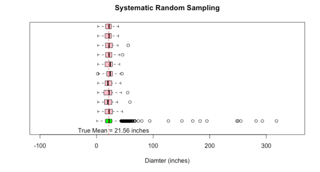
$\mu$ = 21.56 inches

$\sigma^{2}$ = 81.96 $inches^{2}$

$\sigma$ = 9.05 inches

She also noticed that there is a column for whether or not the tree is damaged due to lighting. She computed the true proportion of this.

p = 0.14

Then, as she always does, created a boxplot to check out the full distribution of the data.

“What about Manhattan,” she thought. You are not living in the city if you are not from Manhattan. So she counts the number of trees in each borough and their percentages.

## Count the number of trees in each borough ##
 manhattan_index = which(lpt$borocode==1)
 bronx_index = which(lpt$borocode==2)
 brooklyn_index = which(lpt$borocode==3)
 queens_index = which(lpt$borocode==4)
 staten_index = which(lpt$borocode==5)

 n_manhattan = length(manhattan_index)
 n_bronx = length(bronx_index)
 n_brooklyn = length(brooklyn_index)
 n_queens = length(queens_index)
 n_staten = length(staten_index)

 n_boro = c(n_manhattan,n_bronx,n_brooklyn,n_queens,n_staten)
 barplot(n_boro)

 p_boro = (n_boro/N)
 barplot(p_boro,names.arg = c("Manhattan","Bronx", "Brooklyn", "Queens", "Staten Island"),font=2)

“Hmm 🙁 Let Manhattan at least have the old trees,” she prays and types the following lines to create a map of the trees and their diameters. She also wants to check where the damaged trees are.

There are some libraries required for making maps in R. If you don’t have them, you should install first using install.packages() command.

Jenny is plotting the diameter. plotvar.
The other lines are cosmetics, liners, lipsticks, and blush.

## Plot of London planetrees ##
 library(maps)
 library(maptools)
 library(RColorBrewer)
 library(classInt)
 library(gpclib)
 library(mapdata)
 library(fields)

 par(mfrow=c(1,2))
# plot 1: diameter
 plotvar <- lpt_true_distribution_diam
 
 nclr <- 6 # Define number of colours to be used in plot
 
 plotclr <- brewer.pal(nclr,"Greens") # Define colour palette to be used

# Define colour intervals and colour code variable for plotting
 class <- classIntervals(plotvar, nclr, style = "quantile")

 colcode <- findColours(class, plotclr)

 plot(lpt$longitude,lpt$Latitude,cex=0.15,pch=15, col = colcode, xlab="",ylab="",axes=F,font=2,font.lab=2)

 map("county",region="New York",add=T)
 box()

 title("London Planetrees")
 legend("topleft", legend = names(attr(colcode, "table")), fill = attr(colcode, "palette"), cex = 1, bty = "n",title="Diameter (inches)")

# plot 2: show damaged trees
 plotvar <- lpt_true_distribution_diam
 ind_1 = which(lpt$brnch_ligh=="Yes")

 nclr <- 6 # Define number of colours to be used in plot

 plotclr <- brewer.pal(nclr,"Greens") # Define colour palette to be used

# Define colour intervals and colour code variable for plotting
 class <- classIntervals(plotvar, nclr, style = "quantile")

 colcode <- findColours(class, plotclr)

 plot(lpt$longitude,lpt$Latitude,cex=0,pch=15, col = colcode, xlab="",ylab="",axes=F,font=2,font.lab=2)

 points(lpt$longitude[ind_1],lpt$Latitude[ind_1],pch=20,cex=0.1)

 map("county",region="New York",add=T)
 box()

 title("London Planetrees - Damaged")

The older trees belong mostly to Queens and Brooklyn; so do the damaged trees.

“This will make for a nice example of sampling bias, confidence intervals, and sampling strategies,” she thought as she noticed that the trees with smaller diameters are in Manhattan.

“If we only sample from Manhattan, it will clearly result in a bias in estimation of the population characteristics. Manhattan sample is not fully representative of the population or the true distribution,” she thought.

“Let me compare the population to the sample distributions from the five boroughs.”

She first separates the data for each borough and plots them against the true distribution.

## Breakdown by Borough
 lpt_manhattan = lpt[manhattan_index,]
 lpt_bronx = lpt[bronx_index,]
 lpt_brooklyn = lpt[brooklyn_index,]
 lpt_queens = lpt[queens_index,]
 lpt_staten = lpt[staten_index,]

# Plotting the population and borough wise samples ##
boxplot(lpt$tree_dbh,horizontal=T,xlim=c(0,7),ylim=c(-100,350),col="green",xlab="Diamter (inches)")

 boxplot(lpt_manhattan$tree_dbh,horizontal = T,add=T,at=2,col="red")
 text(-50,2,"Manhattan")

 boxplot(lpt_bronx$tree_dbh,horizontal = T,add=T,at=3,col="pink")
 text(-50,3,"Bronx")

 boxplot(lpt_brooklyn$tree_dbh,horizontal = T,add=T,at=4)
 text(-50,4,"Brooklyn")

 boxplot(lpt_queens$tree_dbh,horizontal = T,add=T,at=5)
 text(-50,5,"Queens")

 boxplot(lpt_staten$tree_dbh,horizontal = T,add=T,at=6)
 text(-60,6,"Staten Island")

 abline(v=lpt_true_mu,lty=2)
 text(30,0,"True Mean = 21.56 inches")

“Brooklyn, Queens and Staten Island resemble the population distribution. Manhattan and the Bronx are biased. If we want to understand the population characteristics, we need a random sample that covers all the five boroughs. The data seems to be stratified. Why don’t I sample data using different strategies and see how closely they represent the population,” she thought.

Simple Random Sampling

She starts with simple random sampling.

“I will use all five boroughs as my sampling frame. Each of these 87014 trees has an equal chance of being selected. Let me randomly select 30 trees from this frame using sampling without replacement. To show the variety, I will repeat this 10 times.”

She types up a few lines to execute this strategy.

# 1: Simple Random Sample
 population_index = 1:N

 ntimes = 10
 nsamples = 30

 simple_random_samples = matrix(NA,nrow=nsamples,ncol=ntimes)
 for (i in 1:ntimes)
 {
   # a random sample of 30 # 
   sample_index = sample(population_index,nsamples,replace=F)
   simple_random_samples[,i] = lpt$tree_dbh[sample_index]
 }

boxplot(lpt$tree_dbh,horizontal=T,xlim=c(0,11),ylim=c(-100,350),col="green",xlab="Diamter (inches)",main="Simple Random Sampling")

 boxplot(simple_random_samples,horizontal = T,boxwex=0.5,add=T,at=c(2:11),col="pink")

 abline(v=lpt_true_mu,lty=2,col="red")
 text(30,0,"True Mean = 21.56 inches")

The sampling is done ten times. These ten samples are shown in the pink boxes against the true distribution, the green box.

Most of the samples cover the true distribution. It is safe to say that the simple random sampling method is providing a reasonable representation of the population.

Stratified Random Sampling

“Let me now divide the population into strata or groups. I will have separate sampling frames for the five boroughs and will do a simple random sampling from each stratum. Since I know the percentages of the trees in each borough, I can roughly sample in that proportion and combine all the samples from the strata into a full representative sample. An inference from this combined samples is what has to be done, not on individual strata samples.”

# 2: Stratified Random Sample
 population_index = 1:N

 ntimes = 10
 nsamples = 100

 stratified_random_samples = matrix(NA,nrow=nsamples,ncol=ntimes)
 for (i in 1:ntimes)
 {
   # Manhattan # 
   ns_manhattan = round(nsamples*p_boro[1])   
   ns_bronx = round(nsamples*p_boro[2])
   ns_brooklyn = round(nsamples*p_boro[3])   
   ns_queens = round(nsamples*p_boro[4])
   ns_staten = nsamples - sum(ns_manhattan,ns_bronx,ns_brooklyn,ns_queens)
 
   sample_manhattan = sample(manhattan_index,ns_manhattan,replace=F)
   sample_bronx = sample(bronx_index,ns_bronx,replace=F)
   sample_brooklyn = sample(brooklyn_index,ns_brooklyn,replace=F)
   sample_queens = sample(queens_index,ns_queens,replace=F)
   sample_staten = sample(staten_index,ns_staten,replace=F)
 
   full_sample = c(lpt$tree_dbh[sample_manhattan],lpt$tree_dbh[sample_bronx],lpt$tree_dbh[sample_brooklyn],lpt$tree_dbh[sample_queens],lpt$tree_dbh[sample_staten])
   
   stratified_random_samples[,i] = full_sample
 }

boxplot(lpt$tree_dbh,horizontal=T,xlim=c(0,11),ylim=c(-100,350),col="green",xlab="Diamter (inches)",main="Stratified Random Sampling")

boxplot(stratified_random_samples,horizontal = T,boxwex=0.5,add=T,at=c(2:11),col="pink")

 abline(v=lpt_true_mu,lty=2,col="red")
 text(30,0,"True Mean = 21.56 inches")

Again, pretty good representation.

She was curious as to where Manhattan is in these samples. So she types a few lines to create this simple animation.

## Animation ##
 for (i in 1:10)
 {
 boxplot(lpt$tree_dbh,boxwex=0.3,horizontal=T,xlim=c(0,2),ylim=c(0,350),col="green",xlab="Diamter (inches)",main="Stratified Random Sampling")

   abline(v=lpt_true_mu,lty=2,col="red")
   text(50,0,"True Mean = 21.56 inches")
   legend(250,2,cex=0.76,pch=0,col="red","Manhattan")
   
stripchart(stratified_random_samples[6:100,i],add=T,at=1.5,cex=0.6,col="blue")

stripchart(stratified_random_samples[1:5,i],add=T,at=1.5,cex=0.75,col="red")

Sys.sleep(1)
 }

The animation is showing the samples each time. Manhattan samples are shown in red. Did you notice that the Manhattan samples are mostly from the left tail? Unless it is combined with the other strata, we will not get a full representative sample.

Cluster Random Sampling

“Both of these methods seem to give good representative samples. Let me now check the cluster random sampling method. We have the zip codes for each tree. So I will imagine that each zip code is a cluster and randomly select some zip codes using the simple random sampling method. All the trees in these zip codes will then be my sample.”

This is her code for the cluster sampling method. She first identifies all the zip codes and then randomly samples from them.

# 3: Cluster Random Sample
 zips = table(lpt$zipcode)
 list_zips = as.numeric(names(zips))
 list_zips = list_zips[-1]

 ntimes = 10
 nsamples = 10

 cluster_random_samples =  NULL
 for (i in 1:ntimes)
 {
   cluster_index = sample(list_zips,nsamples,replace=F)
   cluster_sample = NULL
   for (j in 1:length(cluster_index))
   {
     ind = which(lpt$zipcode==cluster_index[j])
     cluster_sample = c(cluster_sample,lpt$tree_dbh[ind])
   }
   cluster_random_samples = cbind(cluster_random_samples,cluster_sample)
 }
 boxplot(lpt$tree_dbh,horizontal=T,xlim=c(0,11),ylim=c(-100,350),col="green",xlab="Diamter (inches)",main="Cluster Random Sampling")

 boxplot(cluster_random_samples,horizontal = T,boxwex=0.5,add=T,at=c(2:11),col="pink",axes=F)

 abline(v=lpt_true_mu,lty=2,col="red")
 text(30,0,"True Mean = 21.56 inches")

“Hmm. There seems to be one sample which is biased. It is possible. We could have selected most of the zip codes from Manhattan or the Bronx. Since there is not much variability within these clusters, we could not represent the entire population. There is a risk of running poor inferences if we use this sample. Nevertheless, most times we get a good representative sample.”

Systematic Random Sampling

“Let me also try the systematic random sampling method just for completion. I will select every 870th tree in the line up of 87014 trees. I will do this 10 times moving one up, i.e., for the second try, I will select every 871st tree and so forth. Since I am covering the full range of the data, we should get a good representation.”

She types up a few simple lines.

# 4: Systematic Random Sample
 ntimes = 10
 nsamples = 100
 
systematic_random_samples = NULL
 for (i in 1:ntimes)
 {
   # a random sample of 30 # 
 systematic_index = seq(from = i, to = N, by = round((N/nsamples)))
 systematic_random_samples = cbind(systematic_random_samples,lpt$tree_dbh[systematic_index])
 }

boxplot(lpt$tree_dbh,horizontal=T,xlim=c(0,11),ylim=c(-100,350),col="green",xlab="Diamter (inches)",main="Systematic Random Sampling")

 boxplot(systematic_random_samples,horizontal = T,boxwex=0.5,add=T,at=c(2:11),col="pink",axes=F)

 abline(v=lpt_true_mu,lty=2,col="red")
 text(30,0,"True Mean = 21.56 inches")

Things are good for this too.

“This dataset is an excellent resource to demonstrate so many concepts. I will use it to create a situational analysis for my class. I think I can show this over three weeks. Each week, I will introduce one concept. This Monday, I will take a small sample obtained from the simple random sampling method to the class. With this sample data, I will explain the basics of how to compute and visualize confidence intervals in R. I can also show how confidence intervals are derived using the bootstrap method.
Then, I will send them off on a task, asking them to collect data at random from the city. It will be fun hugging trees and collecting data. I should make sure I tell them that the data has to be collected at random from the entire City, not just a few boroughs. Then, all their samples will be representative, and I can show them the probabilistic interpretation of the confidence intervals, the real meaning.
After this, I will ask them to go out and take the samples again, only this time, I will emphasize that they should collect it from their respective boroughs. This means, the folks who collect data from Manhattan will bring biased samples and they will easily fall out in the confidence interval test. This will confuse them !! but it will give a good platform to explain sampling bias and the various strategies of sampling.”

Someday, I shall be gone; yet, for the little I had to say, the world might bear, forever its tone.

If you find this useful, please like, share and subscribe.
You can also follow me on Twitter @realDevineni for updates on new lessons.

Lesson 79 – Pull yourself up by your bootstraps

Over the past several lessons we have been learning about estimates, standard error of the estimates and confidence interval of the estimates.

We have been using the ‘sample’ to estimate the true value of the parameter. What we estimate from the sample will enable us to obtain the closest answer in some sense for the true unknown population parameter.

For example, the mean $\bar{x}$ , variance $s^{2}$ , or proportion $\hat{p}$ computed from the sample data are good guesses (estimates or estimators) of the mean $\mu$ , variance $\sigma^{2}$ and proportion $p$ of the population.

We also know that when we think of an estimate, we think of an interval or a probability distribution, instead of a point value. The truth may be in this interval if we have good representative samples, i.e., if the sample distribution is similar to the population distribution.

Assumptions or Approximations

In this inferential journey, to compute the standard error or to derive the confidence interval of the estimates, we have been making some assumptions and approximations that are deemed reasonable.

For example, it is reasonable to assume a normal distribution for the sample mean $\bar{x}$ .

$\bar{x} \sim N(\mu, \frac{\sigma}{\sqrt{n}})$

The sample mean is an unbiased estimate of the true mean, so the expected value of the sample mean is equal to the truth. $E[\bar{x}]=\mu$ .

The standard deviation of the sample mean, or the standard error of the estimate is $\frac{\sigma}{\sqrt{n}}$ .

This visual should be handy.

—

To derive the confidence interval of the variance and standard deviation, we assumed that $\frac{(n-1)s^{2}}{\sigma^{2}}$ follows a Chi-square distribution with $(n-1)$ degrees of freedom.

$f(\frac{(n-1)s^{2}}{\sigma^{2}}) = \frac{\frac{1}{2}*(\frac{1}{2} \chi)^{\frac{n-1}{2}-1}*e^{-\frac{1}{2}*\chi}}{(\frac{n-1}{2}-1)!}$

Depending on the degrees of freedom, the distribution of $\frac{(n-1)s^{2}}{\sigma^{2}}$ looks like this.

—

Most recently, we assumed that the estimate for proportion $\hat{p}$ can be approximated by a normal distribution.

$\hat{p} \sim N(p, \frac{p(1-p)}{n})$

We derived the confidence interval of the population proportion as $[\hat{p} - Z_{\frac{\alpha}{2}}\sqrt{\frac{\hat{p}(1-\hat{p})}{n}}, \hat{p} + Z_{\frac{\alpha}{2}}\sqrt{\frac{\hat{p}(1-\hat{p})}{n}}]$ , based on this assumption.

Let’s examine this assumption once again.

In a sample of size n, proportion can be estimated as $\hat{p} = \frac{S_{n}}{n}$ , where $S_{n}$ is the number of favorable instances for the thing we are measuring. $\hat{p}$ can be approximated to a normal distribution since $S_{n}$ can be approximated to a normal distribution.

If we take Bernoulli random variables (0,1) for $X_{1}, X_{2}, X_{3}, …, X_{n}$ , $S_{n} = X_{1} + X_{2} + X_{3} + … + X_{n}$ , the number of successes, follows a Binomial distribution $f(x) = \frac{n!}{(n-x)!x!}p^{x}(1-p)^{n-x}$ .

For a large enough sample size n, the distribution function of $S_{n}$ can be well-approximated by the normal distribution.

Let’s do some experiments and see if this is reasonable.

Look at this animation. I am showing the Binomial probability distribution function for p = 0.5 while n increases from 10 to 100.

It looks like an approximation to a normal distribution is very reasonable.

Now, look at these two animations that show the Binomial probability function for p = 0.1 and p = 0.95, i.e., when p is near the boundaries.

Clearly, the distributions exhibit skew and are not symmetric. An approximation to normal distribution even for large values of n, i.e., a big sample, is not appropriate.

How then can we be confident about the standard error and the confidence intervals?
For that matter, how can we derive the standard error or the intervals of a parameter whose limiting form is not known, or mathematically very complicated?

Enter the Bootstrap

Bradley Efron invented a computer-based method, the bootstrap, for estimating the standard error and the confidence intervals of parameters. There is no need for any theoretical calculations or underlying assumptions regarding the mathematical structure or the type of the distribution of the parameter. Instead, bootstrap samples from the data are used.

What is a bootstrap sample?

Suppose we have a data sample, $x_{1},x_{2}, … ,x_{n}$ , a bootstrap sample is a random sample of size n drawn with replacement from these n data points.

Imagine we have the following data: 28.4, 28.6, 27.5, 28.7, 26.7, 26.3 and 27.7 as the concentration of Ozone measured in seven locations in New York City.

Assuming that each data value is equally likely, i.e., the probability of occurrence of any of these seven data points is 1/7, we can randomly draw seven numbers from these seven values.

Think that you are playing the game of Bingo and these seven numbers are chips in your rolling machine. The only difference is, each time you get a number, record it and put it back in the roller until you draw seven numbers. Sample with replacement.

Since each value is equally likely, the bootstrap sample will consist of numbers from the original data (28.4, 28.6, 27.5, 28.7, 26.7, 26.3 and 27.7), some may appear more than one time, and some may not appear at all in a random sample.

I played this using the roller. Here is a bootstrap sample from the original numbers.

As you can see, 28.4 appeared one time, 28.6, 27.5 and 28.7 did not appear, 26.3 appeared 2 times and 27.7 appeared 3 times.

Here are two more bootstrap samples like that.

Basis

The basis for bootstrap samples is that the sample data can be used to approximate the probability distribution function of the population. As you saw before, by putting a probability of 1/n on each data point, we use the discrete empirical distribution $\hat{f}$ as an approximation of the population distribution $f$ .

Take a very simple example of rolling two dice in the game of monopoly. The true probability distribution $f$ of the count (dice 1 + dice 2) is based on the fact that there are 11 possible outcomes and the likelihood of each outcome is the ratio of the total ways we can get the number to 36. An outcome 2 can only be achieved if we get a (1,1). Hence the probability of getting 2 is 1/36.

Suppose we roll the dice a hundred times and record the total count, we can use the observed frequencies of the outcomes from this sample data to approximate the actual probability distribution.

Look at these 100 counts as outcomes of rolling two dice 100 times.

The frequency plot shown in black lines closely approximates the true frequency shown in red.

The empirical distribution $\hat{f}$ is the proportion of times each value in the data sample $x_{1}, x_{2}, …, x_{n}$ occurs. The observed frequency $\hat{f}$ is a sufficient statistic for the true distribution $f$ with an assumption that the data have been generated by random sampling from the true distribution $f$ . All the information of the true distribution $f$ is contained in the empirical distribution $\hat{f}$ .

An unknown population distribution $f$ has produced the observed data $x_{1}, x_{2}, …, x_{n}$ . We can use the observed data to approximate $f$ by its empirical distribution $\hat{f}$ and then use the empirical distribution to generate bootstrap replicates of the data. Since $f$ generated x, $\hat{f}$ can be used to generate the bootstrap samples.

$f$ has given $x_{1}, x_{2},…, x_{n}$ can be used to estimate $\hat{f}$ will be used to generate a $bootstrapsample$ .

This is the basis.

Bootstrap Replicates

Once we generate enough bootstrap samples, we can use the estimators (formula to estimate the parameter) on these samples. For example, if we want to represent the true population mean $\mu$ , we can apply the equation for the sample mean $\bar{x} = \frac{1}{n}{\displaystyle \sum_{i=1}^{n}x_{i}}$ on each of these bootstrap samples to generate bootstrap replicates of the mean.

If we want to represent the true population variance using an interval, we can apply $s^{2} = \frac{1}{n-1}\sum_{i=1}^{n}(x_{i}-\bar{x})^{2}$ on these bootstrap samples to generate replicates of the variance.

Likewise, if we want an interval for the true proportion, we apply $\hat{p} = \frac{S_{n}}{n}$ on the bootstrap samples to get replicates of the proportion.

Each bootstrap sample will produce a replicate of the parameter. Efron prescribes anywhere between 25 to 200 bootstrap replications for a good approximation of the limiting distribution of the estimate. As the number of bootstrap replicates approaches infinity, the standard error as measured by the standard deviation of these replicates will approach the true standard error.

Let’s look at the bootstrap replicates of the sample mean and the sample standard deviation for the Ozone data for which we used the Bingo machine to generate the bootstrap samples. In a later coding lesson, we will learn how to do it using simple functions in RStudio.

For bootstrap sample 1, the sample mean is 27.26 and the sample standard deviation is 0.82.

For bootstrap sample 2, the sample mean is 27.61 and the sample standard deviation is 0.708.

I do this 200 times. Here is how the distribution of the sample mean ( $\bar{x}$ ) obtained from 200 bootstrap replicates looks like.

Here is the distribution of the sample standard deviation.

Like this, we can develop the intervals of any type of parameters by applying the relevant estimator on the bootstrap sample.

Bootstrap confidence interval

Finally, we can use the percentiles of the bootstrap replicates as the confidence limits of the parameter.

Take a 90% confidence interval for instance. From the bootstrap replicates, we can say that there is a 90% probability that the true mean $\mu$ will be between $\bar{x}_{[5]}$ and $\bar{x}_{[95]}$ , the 5th and the 95th percentiles of the bootstrap replicates.

$P(\bar{x}_{[5]} \le \mu \le \bar{x}_{[95]}) = 0.90$

For the Ozone example, the 90% confidence interval of the true mean is [27.114, 28.286] and the 90% confidence interval of the true standard deviation is [0.531 1.087].

Look at these plots.

We can define a $100(1-\alpha)%$ bootstrap confidence interval for the true mean $\mu$ as $[l, u] = [\bar{x}_{[\alpha]}, \bar{x}_{[1-\alpha]}]$ .

There are many more uses of the bootstrap, and we will have much fun with it in due course.

But for today, let’s end with Efron’s statement on what other names were suggested to him for his method.

“I also wish to thank the many friends who suggested names more colorful than Bootstrap, including Swiss Army Knife, Meat Axe, Swan-Dive, Jack-Rabbit, and my personal favorite, the Shotgun, which, to paraphrase Tukey, “can blow the head off any problem if the statistician can stand the resulting mess.””

If you find this useful, please like, share and subscribe.
You can also follow me on Twitter @realDevineni for updates on new lessons.

Category: Sampling Strategies

Lesson 98 – The Two-Sample Hypothesis Tests using the Bootstrap

Two-Sample Hypothesis Tests – Part VII

What do we know so far?

Enter the Bootstrap

Using the Bootstrap for Two-Sample Hypothesis Tests

Manhattan Bridge vs. Williamsburg Bridge

Lesson 83 – The trees of New York

Simple Random Sampling

Stratified Random Sampling

Cluster Random Sampling

Systematic Random Sampling

Lesson 79 – Pull yourself up by your bootstraps

Assumptions or Approximations

—

—

Enter the Bootstrap

What is a bootstrap sample?

Basis

Bootstrap Replicates

Bootstrap confidence interval

Enjoy this blog? Please spread the word :)