J: I believe my decision making has improved. I react based on probability.
D: Great. Assuming you are making decisions for your benefit, in the long run, you will be better off. Probability is the guiding force.
J: I am visiting Vegas next week. I want to use “the force” to outwit the house.
D: For that, the necessary condition is to know about conditional probability.
J: I know that probability is the long-run relative frequency. But what is conditional probability?
D: Since you are excited about Vegas, let us take the cards example.
Say, we have a deck of cards. If I shuffle and draw a card at random, what is the probability of getting a king?
J: Let me use my probability logic here. I will assume that the 52 cards will make up our sample space. Since there will be 4 kings in a deck of 52 cards, if your shuffling is fair, the likelihood of getting a king is 4/52.
D: Good. Let us call this event A → King.
What are the odds of getting a red card?
J: Since there will be 26 red cards in 52, the odds of getting a red card are 26/52.
D: Exactly. Let us call this event B → Red.
Now, If I draw a card at random, face down, and tell you that it is red, what is the probability that it will be a king?
J: So you are providing me some information about the card?
D: Yes, I am giving you a condition that the card is red.
J: Okay. Under the condition that the card is red, the odds of it being a king should be 2/26.
D: Can you elaborate.
J: Since you told me that the card is red, I only have to see how many kings are there in red cards. The sample space is now 26. There are two red kings. So the probability will be 2/26.
D: Good. Mathematically, this is written as
P(A|B) = P(A ∩ B) / P(B)

or

P(King | Red) = P(King and Red) / P(Red)
P(King and Red) is 2/52. P(Red) is 26/52. So we get 2/26.
J: I get it. My answer will depend on the condition. Can you provide one more example?
D: Sure. You told me that the probability of getting a king is 4/52. Suppose, this first card is faced up, and I draw another card face down. What is the probability that this second card is a king?
J: Since the first card is on the table and not replaced, the probability that the second card will be a king should be 3/51. Three kings left in the deck of 51.
D: Correct. The outcome of the second card is conditional on the outcome of the first card.
J: This makes perfect sense. If I can practice this counting and conditional probability, I can make some money on blackjack.
D: Yes you can. Knowing conditional probability is the necessary condition.
J: Why do you keep saying “necessary condition”?
D: Probability is your guiding force everywhere else in life.
But in Vegas, Joe Pesci is the force.
If you find this useful, please like, share and subscribe. You can also follow me on Twitter @realDevineni for updates on new lessons.
As I am taking my usual Broadway stroll this morning, I noticed some people immersed in their smartphone, texting or browsing while walking. Guilty as charged. It reminded me of the blog post a few years ago about my memory down the phone lane.
I started paying attention to my surroundings and noticed this kiosk, a free wifi hotspot provided by the City of New York.
So, I used their wifi to look up LinkNYC. Thier description tells me that “LinkNYC is a first-of-its-kind communications network that will replace over 7,500 pay phones across the five boroughs with new structures called Links. Each Link provides superfast, free public Wi-Fi, phone calls, device charging and a tablet for access to city services, maps and directions.”
They have been around since January 2016. I want to know how many such kiosks are there in the City and each borough. They have a map on their website for locating the kiosks, but it is hard for me to count points on a map. My City at service again, I found the entire wifi hotspot locations data on NYC Open Data.
Let us learn some tricks in R while trying to answer this question.
Usual chores.
Step 1: Get the data
I downloaded the hotspot data file from here.
Step 2: Create a new folder on your computer
Let us call this folder “lesson8”. The downloaded data file “Free_WiFi_Hotspots_09042005.csv” is saved in this folder.
Step 3: Create a new code in R
Create a new code for this lesson – “lesson8_code.R”.
Step 4: Choose your working directory
In this lesson, we have a folder named “lesson8”. So we should tell R that “lesson8” is the folder where the data files are stored. You can do this using the “setwd” command. If you followed the above steps and if you type list.files() in the console, you would see “lesson8_code.R” and “Free_WiFi_Hotspots_09042005.csv” on the screen as the listed files in your folder.
Step 5: Read the data into R workspace
Since we have a comma separated values file (.csv), we can use the “read.csv” command to read the data file into R workspace. Type the following line in your code and execute it. Why am I giving header=TRUE in the command?
# Read the data file #
wifi_data = read.csv("Free_WiFi_Hotspots_09042005.csv",header=T)
Step 6: Use the data to answer the questions
It will be helpful to learn some new concepts in R coding before we address the actual kiosk problem. The for loop, storing values in matrices, and if else statements.
Loops: Do you remember your fun trips to batting cages? Just like the pitching machine is set up to pitch the baseball, again and again, you can instruct R to run commands again and again. For example, if you want to print NYC ten times, instead of typing it ten times, you can use the for loop.
You are instructing R to print NYC ten times by using the command for (i in 1:10). The lines within the {} will be repeated ten times. Select the lines and hit the “Run” button to execute. You will see this in the console screen.
Matrices: I am sure you have been to a college or public library to check out books. Can you remember the bookcases that store the books? Just like a bookshelf with many horizontal and vertical dividers, in R you can create matrices with many rows and columns and use them to store values (numbers or text). Type the following lines in your code.
# create an empty matrix of NA in 10 rows and 1 column
x = matrix(NA,nrow=10,ncol=1)
print(x)
You can create an empty matrix called x with ten rows and 1 column. The NA is a space. We can fill this space with numbers later.
Now imagine we combine the above instructions, we want to store NYC in a matrix or shelf; like printing NYC ten times on a paper and arranging them in each row of a bookshelf. Type the following lines and see the results for yourself. The empty matrix x will be filled with NYC using the for loop.
# store NYC in a matrix of 10 rows and 1 columns
x <- matrix(NA,nrow=10,ncol=1)
for (i in1:10)
{
x[i,1] = "NYC"
}
print(x)
If Else Statement: Do you remember cleaning your room on a Sunday? Recall those terrible times for a minute and think about what you did. If you find a book lying around, you would have put it in the bookshelf. If you find a toy, you may have put it in your toy bag. If you find a shirt or a top, it goes into the closet. The if else statement works exactly like this. You are instructing R to perform an action if some condition is true, else some other work.
if (condition) {statement} else {statement}
For example, let us say we want to print a number 1 if the 10th row of the matrix x is “NYC”; else, we want to print a number 0. We can do this using the following lines.
The conditon is x[10,1] == “NYC”, the output is printing 1 or 0.
Okay, let us get back to the wifi hotspot business. If you look at the Free_WiFi_Hotspots_09042005.csv file, you will notice that the 4th column is an indicator for which borough the kiosk is in, and the 5th column is the indicator for the service provider. LinkNYC is not the only free wifi provider in the city. Time Warner, AT and T, Cable Vision are some of the other providers.
So here is a strategy or a set of instructions we can give R to see how many LinkNYC kiosks are there is Manhattan. We first check for the total number of kiosks. There are 2061 kiosks in the City (number of rows of the table). Wow..
We look through each row (kiosk) and check if the provider is LinkNYC, and the borough is Manhattan. If it is the case, we assign a 1; else we assign a 0. We count the total number of ones. Here is the code.
## finding NYC LINK kiosks in Manhattan ##
n = nrow(wifi_data)
linknyc_hotspots = matrix(NA,nrow=n,ncol=1)
for (i in1:n)
{
if((wifi_data[i,4]=="MN") & (wifi_data[i,5]=="BETA LinkNYC - Citybridge"))
{linknyc_hotspots[i,1] = 1} else {linknyc_hotspots[i,1] = 0}
}
sum(linknyc_hotspots)
Notice what I did.
I first created an empty matrix with 2061 rows and 1 column.
Using the for loop, I am looking through all the rows.
For each row, I have a condition to check – the provider is LinkNYC, and the borough is Manhattan. Notice how I check for the conditions using the (condition 1) & (condition 2). If these conditions are true, I will fill the empty matrix with 1, else, I will fill it with 0.
In the end, I will count the total number of ones.
There are 521 LinkNYC kiosks in Manhattan. Still Wow..
Can you now tell me how many LinkNYC kiosks are there in Brooklyn and how many Time Warner Cable kiosks are there in the Bronx?
While you tell me the answer, I want to sing Frank Sinatra for the rest of the day. I love my City. I can take long walks; I can be car free; I can get free wifi access; I can even get free data to analyze.
Wait, maybe I should not use “free” in my expression of the love for the City.
April 18th is fast approaching.
If you find this useful, please like, share and subscribe. You can also follow me on Twitter @realDevineni for updates on new lessons.
“Professor, I am nervous about the test.”
“Professor, how should we study for the test?”
“Professor, what questions can we expect on the test?”
“Professor, what formulas will you provide on the test?”
“Professor, I am getting stressed out.”
I want to respond.
“I know how you feel.”
This response will not help because if I was taking a test, and I was nervous, I don’t need confirmation from my professor that he knows how I feel.
“I have been in your shoes.” or “Been there, done that.”
Really… besides not helping, this response will make them angry. I am not in their shoes now, and who cares if I have done it before.
“You are on your own. Go figure it out.”
No, I am on their side, and we are taking down the data analysis beast together.
Since the responses are not working, I provide a way to think probabilistically.
Let us say there are 15 questions that you need to study for the test. These 15 questions are our sample space.
The probability of the sample space is 1 — Probability Axiom 1
The likelihood of being tested from these 15 questions is 1. You cannot escape this unless you decide to skip the test.
Let us now group these questions into concepts. Suppose there are three concepts, Concept A, Concept B and Concept C. Go through each question and identify to which concept it belongs. For instance,
We see that six questions belong to concept A, seven questions belong to concept B, and five questions belong to concept C. Three questions have both concept A and concept B. Switch to a visual mode – you will see this.
By now, you should know that the probability of getting a question from concept A is 6/15 = 0.4,the probability of getting a question from concept B is 7/15 = 0.466, and the probability of getting a question from concept C is 5/15 = 0.333.
Underlying this number is the rule that the probability of any event in the sample space is between 0 and 1 — Probability axiom 2.
In other words, if there were no questions that belonged to concept A, then, the probability would have been 0 (0/15). If all the 15 questions were from concept A, the probability would have been 1 (15/15).
Let us now think about the probability of getting a question from concept A or concept C. 11 questions in total belong to concept A or concept C; six from A and five from C. Hence, the probability of getting a question from concept A or concept C is
In this example, there are no questions that have both concept A and concept C. They are disjoint sets. For disjoint or mutually exclusive events, the probability that one or the other of the two events occurs is the sum of their individual probabilities — Probability axiom 3.
Let us extend this understanding to the probability of getting a question from concept A or concept B. if you look at the Venn diagram above; you will see that there are 3 + 3 + 4 questions that are either concept A or concept B or both. Hence, the probability of getting a question from concept A or concept B is
Since three questions belong to both A and B (i.e., the intersection of A and B), it will be sufficient to count them once. In the equation, you are adding the probability of A (6 questions out of 15), to the probability of B (7 questions out of 15), and subtracting the intersection (3 common questions out of 15) to avoid double counting.
Now that the ground rules (Axioms of Probability) are set, all you need to do is calculate the probability of getting exactly one question from binomial distribution in a total of 5 questions and hope your prediction will come true! That was for my friends in the class.
Oh, I love this game. They anticipate my behavior and predict the probability of getting any question. I anticipate that they do this, hence, try to outsmart them.
I get a sense that my folks figured out the pattern here. Beavers are Strivers. Wikipedia also tells me that beavers build dams, canals, and lodges.
If you find this useful, please like, share and subscribe. You can also follow me on Twitter @realDevineni for updates on new lessons.
Let me introduce you to two friends, Joe and Devine.
Joe is a curious kid, funny, feisty and full of questions. He is sharp and engaging and always puts in the honest effort to understand things.
Devine is mostly boring, but thoughtful. He believes in reason and evidence and the scientific method of inquiry.
Joe and Devine stumbled upon our blog and are having a conversation about Lesson 5.
Joe: Have you seen the recent post on data analysis classroom. There was an interesting question on how many warm days are there in February.
Devine: What do you mean by warm? Where is it warm?
Joe: Look, Devine, I know you always want to think from first principles. Can you stop being picky and cut to the chase here.
Devine: Okay, how many warm days are there in February?
Joe: Looks like there were seven warm days last month. That seems like a high number.
Devine: Maybe. Do you know the probability of warm days in February?
Joe: What is “probability“?
Devine: Let us say it is the extent to which something is probable. How likely is a warm day in February? In other words, how frequently will warm day occur in February?
Joe: I can see there are seven warm days in February out of 28 days. So that means the frequency or likeliness is seven in 28. 7/28 = 0.25. So the probability is 25%.
Devine: What you just computed is for February 2017. How about February 2016, 2015, 2014, 2013, … ?
Joe: I see your point. When we compute the frequency, we are trying to see how many times an event (in this case warm day in February) is occurring out of all possibilities for that event.
Devine: Yes. Let us say there is a set of February days; 28 in 2017, 29 in 2016, 28 in 2015, so on and so forth. These are all possible February days. Among all these days, we see how many of them are warm days.
Joe: So you mean what is the frequency in the long run.
Devine: Yes, the probability of an event is its long-run relative frequency.
Joe: Let me get the data for all the years and see how many warm days are there in February.
Devine: That is a good idea. When you get the data, try the following experiment to see how the probability approaches the true probability as you increase the sample space.
Step 1: Compute the number of warm days in February 2017. Let us call this warmdays2017. So the probability of warm days is p = warmdays2017 divided by 28.
Step 2: Compute the number of warm days in February 2016. Let us call this warmdays2016. Using this extended sample size, we calculate the probability of warm days as p = (warmdays2017 + warmdays2016) divided by 57; 28 days in 2017 and 29 days in 2016. Here you have more outcomes (warm days) and more opportunities (February days) for these outcomes.
Step 3: Do this for as many years as you can get data, and make a plot (visual) of growing years and true probability.
Joe: I got the logic, but this looks like a lot of counting for me. Is there an easier way?
Devine: R can help you do this easily. Perhaps, you can wait till the data analysis guy posts another lesson of tricks in R. For now, let me help you.
Joe: Great.
Devine: Okay, here is what I got after running this experiment.
Joe: This is pretty. Let me try to interpret it. On the x-axis you have Years up to; and the axis is showing 2017, 2016, …, 1949. So that means, in each step, you are considering the data up to that year — up to 2017, up to 2016, up to 2015 so on and so forth. On the y-axis, you have the probability of warm days in February. At each step, you are computing the probability with new sample size, so you have a better idea of the likelihood of warm days since there are more outcomes and opportunities.
Devine: Exactly. What else do you observe?
Joe: There is a red line somewhere around 0.02, and the probabilities are approaching this red line as we have more sample size.
Devine: Great, the red line is at 0.027, and the long run relative frequency — Probability of warm days in February is 0.027. Notice that the probability does not vary much, and looks like a stable line after you go up to 2000s. This is telling us that we need enough sample size to get a reliable measure of the probability.
Joe: What happens to the probability if we have 50 more years of data?
Devine: ah…
Joe: Wait, I thought the probability based on 2017 data is 0.25. Why is the first point on the plot at 0.15?
Devine: Joe, you are the curious kid.. Go figure it out.
In case you are wondering who Devine is,
It’s probably me.
If you find this useful, please like, share and subscribe. You can also follow me on Twitter @realDevineni for updates on new lessons.
I am staring at my MacBook, thinking about the opening lines. As my mind wanders, I look over the window to admire the deceivingly bright sunny morning. The usually pleasant short walk to the coffee shop was rather uncomfortable. I ignored the weatherman’s advice that it will feel like 12 degrees today. Last week, my friend expressed his concern that February was warm. I begin to wonder how often is Saturday cold and how many days in the last month were warm. Can I look at daily temperature data and find these answers? Maybe, if I can get the data, I can ask my companion R to help me with this. Do you think I can ask R to find me the set of all cold days, the set of all warm days and the set of cold Saturdays? Let us check out. Work with me using your RStudio program.
Step 1: Get the data
I obtained the data for this review from the National Weather Service forecast office, New York. For your convenience, I filtered the data with our goals in mind. You will notice that the data is in a table with rows and columns. Each row is a day. The columns indicate the year, month, day, its name, maximum temperature, minimum temperature and average temperature. According to the National Weather Service’s definition, the maximum temperature is the highest temperature for the day in degrees Fahrenheit, the minimum temperature is the lowest temperature for the day, and the average temperature for the day is the rounded value of the average of the maximum and the minimum temperature.
Step 2: Create a new folder on your computer
When you are working with several data files, it is often convenient to have all the files in one folder on your computer. You can instruct R to read the input data from the folder. Download the “nyc_temperature.txt” file into your chosen folder. Let us call this folder “lesson5”.
Step 3: Create a new code in R
Create a new code for this lesson. “File >> New >> R script”.
Save the code in the same folder “lesson5” using the “save” button or by using “Ctrl+S”. Use .R as the extension — “code_lesson5.R”. Now your R code and the data file are in the same folder.
Step 4: Choose your working directory
Make it a practice to start your code with the first line instructing R to set the working directory to your folder. In this lesson, we have a folder named “lesson5”. So we should tell R that “lesson5” is the folder where the data files are stored. You can do this using the “setwd” command.
The path to the folder is given within the quotes. Execute the line by clicking the “Run” button on the top right. When this line is executed, R will read from “lesson5” folder. You can check this by typing “list.files()” in the console. The “list.files()” command will show you the files in the folder. If you followed the above steps, your would see “code_lesson5.R” and “nyc_temperature.txt” on the screen as the listed files in your folder.
Step 5: Read the data into R workspace
The most common way to read the data into R workspace is to use the command “read.table”. This command will import the data from your folder into the workspace. Type the following line in your code and execute it.
Notice that I am giving the file name in quotes. I am also telling R that there is a header (header=TRUE) for the data file. The header is the first row of the data file, the names of each column. If there is no header in the file, you can choose header=FALSE.
Once you execute this line, you will see a new name (nyctemperature) appearing in the environment space (right panel). We have just imported the data file from the “lesson5” folder into R.
Step 6: Use the data to answer the questions
Let us go back to the original questions. How many days in the last month were warm, and how often is Saturday cold.
Let us call data for the months of January and February as the sample space S. S is the set of all data for January and February. Type the following lines in your code to define sample space S.
Notice that S is a table/matrix with rows and columns. In R, S[1,1] is the element in the first row and first column. S[1,7] is the element in the first row and seventh column, i.e. the average temperature data for the first day. If you want to choose the entire first row, you can use S[1, ] (1 followed by a comma followed by space within the square brackets). If you want to select an entire column, for instance, the average temperature data (column 7), you can use S[ ,7] (a space followed by a comma followed by the column number 7).
To address the first question, we should identify warm days in February. We need to define a set A for all February data, and a set B for warm days.
Recall lesson 4 and check whether A and B are subsets of S.
Type the following lines in your code to define set A.
S[ ,2] is selecting the second column (month) from the sample space S. The “which(S[ ,2]==2)” will identify which rows in the month column are equal to 2, i.e. we are selecting the February days. Notice that A will give you numbers 32 to 59, the 32nd row (February 1) to 59th row (February 28) in the data.
Next, we need to define set B as the warm days. For this, we should select a criterion for warm days. For simplicity, let us assume that a warm day is any day with an average temperature greater than or equal to 50 degrees F. Let us call this set B = set of all warm days. Type the following lines in your code and execute to get set B.
S[ ,7] is selecting the 7th column (average temperature) from the sample space S. The “which(S[ ,7]>=50)” will identify which rows have an average temperature greater than or equal to 50. Notice that B will give your numbers 12, 26, 39, 50, 53, 54, 55, 56, and 59; the rows (days) when the average temperature is greater than or equal to 50 degrees F. February 28th, 2017 had an average temperature of 53 degrees F. I believe it was that day when my friend expressed his unhappiness about the winter being warm!
Now that we have set A for all February data, and set B for warm days, we need to identify how many elements are common in A and B; what is the intersection of A and B. The intersection will find the elements common to both the sets (Recall Lesson 4 – intersection = players interested in basketball and soccer). Type the following line to find the intersection of A and B.
The “intersect” command will find the common elements of A and B. You will get the numbers 39, 50, 53, 54, 55, 56, and 59. The days in February that are warm. Seven warm days last month — worthy of my friend’s displeasure.
Can you now tell me how often is Saturday cold based on the data we have? Assume cold is defined as an average temperature less than or equal to 25 degrees F.
Did you realize that I am just whining about Saturday being cold? Check out the “union” command before you sign off.
If you find this useful, please like, share and subscribe. You can also follow me on Twitter @realDevineni for updates on new lessons.
So am I. Aren’t we all? Our brain likes it that way.
Let us activate our visual cortex to learn more about Sets. Imagine that you are taking a headcount for high school or college intramurals. You have players who are interested in basketball and players who are interested in soccer. Some of them are interested in participating in both basketball and soccer.
Let us ask them to organize themselves into the basketball and soccer teams. A simple visual of this would look like:
Let us call our basketball players Team Basket (B). Let us call our soccer players Team Soccer (S). Let us call all of them Team Intramural (I).
If Team Intramural is the set of all players interested in participating in sports, Team Basket and Team Soccer are subsets of Team Intramural. All the players in Team Basket and Team Soccer also belong to Team Intramural.
All players who do not play soccer are the complement of Team Soccer. The complement of a set is used to denote everything but the set.
If you want to know how many players are interested in basketball or soccer, you can visualize the entire space that includes Team Basket or Team Soccer. The union of these two teams or set.
If you want to know how many players are interested in basketball and soccer, you can visualize the space that includes players that like to participate in both. The individuals who intersect the two teams.
If you want to take a count of players interested in only one sport but not both, you can visualize a space that includes players that like basketball or players that like soccer, but the players that like both will miss out. This grouping is also called symmetric difference, or the Union – Intersection.
Now imagine another class of students approached you inquiring about field hockey. Let us call this new team, Team Hockey. Team Hockey will become a subset of Team Intramural. However, the players of Team Hockey and the players of Team Soccer do not have anything in common. They are mutually exclusive. They are disjoint. They don’t cross lines — their intersection is 0.
Next week, we will learn how to use real data in RStudio, how to categorize the data into sets, and how to check for intersections, unions, and exclusiveness. In the meantime, try to visualize how our players and teams fit these other Set Properties.
If the union of all sets makes up the entire space, then the sets are collectively exhaustive. Our Team Soccer, Team Basketball, and Team Hockey are collectively Team Intramural (Exhaustive).
I finally think my students got the idea of mutually exclusive and collectively exhaustive sets when I told them that the mid terms are mutually exclusive, but the final exam is collectively exhaustive !! They must have visualized the final.
If you find this useful, please like, share and subscribe. You can also follow me on Twitter @realDevineni for updates on new lessons.
We begin our quest with the idea of classifying things. Whether it is Aristotle grouping animals into those living in water and those living on land, or you and me grouping our daily activities into those best done in the morning and those best done in the evening, we are all obsessed with putting things in order – into blocks — groups — SETS.
Math puritans can start with Georg Cantor’s Set Theory. Others can think of SET as a collection of distinct elements.
The fruit basket in your house is a set of fruits consisting of apples, bananas, and grapes – {apple, banana, grapes}.
After work, you can visit a local hangout place where you find a set of people interested in alcohol or food or both.
The vowels in English alphabets are a set {a, e, i, o, u}. The English alphabets are a set {a, b, c, …, x, y, z}.
The outcomes of a coin toss are a set {Head, Tail}.
In the game of Monopoly, you move by the outcomes of the dice. These outcomes are a set of number combinations – {(1,1), (1,2) … (6,6)}.
We all tried rolling a double to get out of jail. Did you know that the odds of getting out of jail by rolling a double are only 16.6%?
There are six possible doubles (see the red background combinations along the diagonal – {(1,1), (2,2), (3,3), (4,4), (5,5), (6,6)}) when you roll two dice. The entire set of possible combinations are 36. The odds are 6/36. Maybe you should have paid the $50 to get out of jail immediately.
Think about sets and possible outcomes in whatever you do this week — Happy President’s Day.
Speaking of Presidents, you should have already imagined a Set of
If you find this useful, please like, share and subscribe. You can also follow me on Twitter @realDevineni for updates on new lessons.
is your companion in this journey through data. It is a software environment that performs the analysis and creates plots for us upon instruction. People who are familiar with computer programming need no introduction. Others who are just getting started with data analysis but are skeptical about computer programming – count the number of 1’s in this data. You will need no more convincing to embrace R.
You can follow these steps to install R and its partner RStudio.
1) Installing R: Use this link https://cran.r-project.org to download and install R on your computer. There are separate download links for Mac, Windows or Linux users.
2) Installing RStudio: Use this link https://www.rstudio.com/products/rstudio/download/ to download and install RStudio on your computer. RStudio will be your environment for coding and visualizations. For RStudio to run, you need to install R; which is why we followed step 1.
Getting started with RStudio
Open RStudio – you should see three panels, the console, environment and history and the files panels.
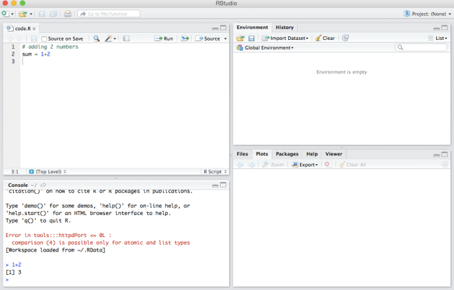
In the console panel, you will get a copyright message and a “>” prompt. Type 1+2 and hit enter here to check that RStudio is working. You should see the number 3 pop up, which means you are ready to go.
Writing your code
You can use a text editor to give instructions to RStudio (writing your code) and save those instructions (saving your code). In the text editor, you can also write comments to help you remember the steps and make it user-friendly and readable. As a simple example, imagine you want to add 2 numbers, 1 and 2 and you want to write instructions for this. You can type
The first line starts with a #; it is a comment — for people to know that you are adding 2 numbers.
The second line is the actual code or instruction to add 1 and 2.
Remember, a well-written code with clear comments is like having good handwriting.
Opening the text editor
Once you load RStudio, go to “File >> New >> R script”.
You will now see the text editor as the 4th panels on RStudio. You can save the code using the “save” button or by using “Ctrl+S”. Use .R as the extension — “code.R”.
Some simple code
Type the following lines in your code and execute them by clicking the “Run” button on the top right.
Shortcut: You can also place the cursor on the line and hit “Ctrl+Enter” if you are using Windows or “Cmd+Enter” if you are using a Mac. Notice the results of your code in the console.
I have more simple instructions for practice here. Copy them to your code and have fun coding.
We will learn data analysis using RStudio. I will provide more coding tricks as we go along.
If you find this useful, please like, share and subscribe. You can also follow me on Twitter @realDevineni for updates on new lessons.
Data is the key to understanding patterns, learning about behaviors, testing your theories, and supporting your arguments. It provides an entry point to get a general idea about anything. Make a commitment to yourself that you will think about data when you see something. Here, I provide some common situations to prime the pump.
Preferred Coffee: I am writing this post from a coffee shop. My favorite coffee is espresso. I am curious about what others visiting this shop prefer. I can either sit all day and watch what they buy (which will get the manager suspicious) or ask the cashier about how many people purchased espresso or other coffee (tell them it’s a scientific experiment first!).
Cars and Tolls: We all waited in line to pay the toll to use the bridge. Friends from the tri-state area are thinking EZPASS. Yes, next time you pass a toll, think about how many cars pass the toll in a day. We can use this data to understand how many people use the bridge and how much revenue it generates.
Fitbit: Look at your Fitbit or smartphone health app. Tell me how many hours your sleep on average.
You get the point.
If you find this useful, please like, share and subscribe. You can also follow me on Twitter @realDevineni for updates on new lessons.
Uncertainties surround us. Understanding where they arise from and recognizing their extent is fundamental to improving our knowledge about anything. This website is all about analyzing the data to interpret the uncertainties. It will contain series of blog posts attempting to explain key ideas in bite sizes. Post your questions in the comments bar. Happy learning!