Another one of those pharmacy umbrellas is resting in peace after yesterday’s Nor’easter. On a day when a trailer toppled on Verazzona bridge, I must be happy it is only my umbrella that blew away and not me. These little things are so soft they can at best handle a happy drizzle.

As per the National Weather Service, winds (gusts) were up to 35 miles per hour yesterday. We are still under a wind advisory as I write this.
My mind is on exploring how many such gusty events happened in the past, what is the wait time between them and more.
I have requested the daily wind gust data for New York City from NOAA’s Climate Data Online.
So, get your drink for the day and fire up your R consoles. Let’s recognize this Nor’easter with some data analysis before it fades away as a statistic. We don’t know how long we have to wait for another of such event. Or do we?
FIRST STEPS
Step 1: Get the data
You can download the filtered data file here.
Step 2: Create a new folder on your computer
Let us call this folder “lesson55.” Save the data file in this folder.
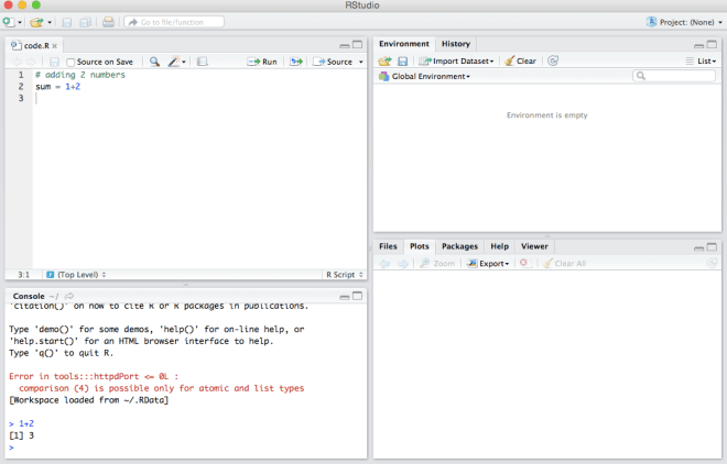
Step 3: Create a new code in R
Create a new code for this lesson. “File >> New >> R script.” Save the code in the same folder “lesson55” using the “save” button or by using “Ctrl+S.” Use .R as the extension — “lesson55_code.R.” Now your R code and the data file are in the same folder.
Step 4: Choose your working directory
“lesson55” is the folder where we stored the data file. Use “setwd(“path”)” to set the path to this folder. Execute the line by clicking the “Run” button on the top right.
setwd("path to your folder")
Step 5: Read the data into R workspace
I have the data in the file named “cp_wind.csv.” I am only showing the wind gust data for the day. The column name (according to NOAA CDO) is WSFG.
WSFG = Peak guest wind speed (miles per hour or meters per second as per user preference)
Type the following line in your code and execute it. Use header=TRUE in the command.
#### Read the file ####
cp_data = read.csv("cp_wind.csv",header=TRUE)
Counts – Poisson Distribution
There is data from 1984 to 2017, 34 years.
Execute the following line in your code to count the total number of days when wind gust exceeded 35 mph.
# Select Wind Gust data > 35 mph from the file #
gust_events = length(which(cp_data$WSFG > 35))
The which command outputs the index of the row that is greater than 35 mph. The length command counts the number of such days.
There are 653 such events in 34 years, an average of 19.20 events per year.
Let’s count the events each year from 1984 to 2017.
Write the following lines in your code.
# Count the number of events each year #
years = range(cp_data$Year)

number_years = diff(years) + 1

gust_counts_yearly = matrix(NA,nrow=number_years,ncol=1)

for (i in 1:number_years)
{
 year = 1983 + i
 index = which(cp_data$Year == year)
 gust_counts_yearly[i,1] = length(which(cp_data$WSFG[index] > 35))
}

plot(1984:2017,gust_counts_yearly,type="o",font=2,font.lab=2,xlab="Years",ylab="Gust Counts")

hist(gust_counts_yearly)
lambda = mean(gust_counts_yearly)
Assuming that we can model the number of gust events each year as a Poisson process with the rate you estimated above (19.2 per year), we can generate Poisson random numbers to replicate the number of gust events (or counts) in a year.
If we generate 34 numbers like this, we just created one possible scenario of yearly gust events (past or future).
Run the following line in your code.
# create one scenario #
counts_scenario = rpois(34,lambda)
Now, you must be wondering how the command rpois works? What is the mechanism for creating these random variables?
To understand this, we have to start with uniform distribution and the cumulative density functions.
 is an increasing function of
  , and we know that
  . In other words, is uniformly distributed on [0, 1].
For any uniform random variable u, we can say  since
since  for uniform distribution.
Using this relation, we can obtain x using the inverse of the function F.  .
.
If we know the cumulative distribution function F of a random variable X, we can obtain a specific value from this distribution by solving the inverse function for a uniform random variable u. The following graphic should make it clear as to how a uniform random variable u maps to a random variable x from a distribution. rpois implicitly does this.

Uniform Distribution
Do you remember lesson 42? Uniform distribution is a special case of the beta distribution with a standard form
 for
for  .
.
a and b are the parameters that control the shape of the distribution. They can take any positive real numbers; a > 0 and b > 0.
c is called the normalizing constant. It ensures that the pdf integrates to 1. This normalizing constant c is called the beta function and is defined as the area under the graph of  between 0 and 1. For integer values of a and b, this constant c is defined using the generalized factorial function.

Substitute a = 1 and b = 1 in the standard function.


A constant value 1 for all x. This flat function is called the uniform distribution.
In lesson 42, I showed you an animation of how the beta function changes for different values of a and b. Here is the code for that. You can try it for yourself.
I am first holding b constant at 1 and varying a from 0 to 2 to see how the function changes. Then, I keep a at 2 and increase b from 1 to 2. If you select the lines altogether and run the code, you will see the plot domain running this animation. The Sys.sleep (1) is the control to hold the animation/loop speed.
### Beta / Uniform Distribution ###

### Animation ###

a = seq(from = 0.1, to = 2, by = 0.1)
b = 1

x = seq(from = 0, to = 1, by = 0.01)
for (i in 1:length(a))
{
 c = factorial(a[i]+b-1)/(factorial(a[i]-1)*factorial(b-1))
 fx = c*x^(a[i]-1)*(1-x)^(b-1)

 plot(x,fx,type="l",font=2,font.lab=2,ylab="f(x)",ylim=c(0,5),main="Beta Family")
 txt1 = paste("a = ",a[i])
 txt2 = paste("b = ",b)

 text(0.6,4,txt1,col="red",font=2)
 text(0.6,3.5,txt2,col="red",font=2)

 Sys.sleep(1)
}

a = 2
b = seq(from = 1, to = 2, by = 0.1)

x = seq(from = 0, to = 1, by = 0.01)
for (i in 1:length(b))
{
 c = factorial(a+b[i]-1)/(factorial(a-1)*factorial(b[i]-1))
 fx = c*x^(a-1)*(1-x)^(b[i]-1)

 plot(x,fx,type="l",font=2,font.lab=2,ylab="f(x)",ylim=c(0,5),main="Beta Family")
 txt1 = paste("a = ",a)
 txt2 = paste("b = ",b[i])

 text(0.6,4,txt1,col="red",font=2)
 text(0.6,3.5,txt2,col="red",font=2)

 Sys.sleep(1)
}
You should see this running in your plot domain.

Exponential Distribution
Let’s get back to the gusty winds.
Remember what we discussed in lesson 43 about the exponential distribution. The time between these gusty events (wind gusts > 35 mph) follows an exponential distribution.

Here is the code to measure the wait time (in days) between these 653 events, plot them as a density plot and measure the average wait time between the events (expected value of the exponential distribution).
### Exponential Distribution ###

# Select the indices of the Wind Gust data > 35 mph from the file #
library(locfit)

gust_index = which(cp_data$WSFG > 35)

gust_waittime = diff(gust_index)

x = as.numeric(gust_waittime)
hist(x,prob=T,main="",xlim=c(0.1,200),lwd=2,xlab="Wait time in days",ylab="f(x)",font=2,font.lab=2)
lines(locfit(~x),xlim=c(0.1,200),col="red",lwd=2,xlab="Wait time in days",ylab="f(x)",font=2,font.lab=2)

ave_waittime = mean(gust_waittime)
The first event recorded was on the 31st day from the beginning of the data record, January 31, 1984. A wait time of 31 days. The second event occurred again on day 55, February 24, 1984. A wait time of 24 days. If we record these wait times, we get a distribution of them like this.

Now, let’s generate 34 random numbers that replicate the time between the gusty events.
# Simulating wait times #
simulated_waittimes = rexp(34,lambda)*365

plot(locfit(~simulated_waittimes),xlim=c(0.1,200),col="red",lwd=2,xlab="Wait time in days",ylab="f(x)",font=2,font.lab=2)
rexp is the command to generate random exponentially distributed numbers with a certain rate of occurrence lambda. In our case, lambda is 19.2 per year. I multiplied them by 365 to convert them to wait time in days.
What is the probability of waiting more than 20 days for the next gusty event?
Yes, you’d compute  .
.
In Rstudio, you can use this line.
# Probability of wait time greater than 20 days #
lambda = 1/ave_waittime

1 - pexp(20, lambda)
pexp computes  .
.
Now, imagine we waited for 20 days, what is the probability of waiting another 20 days?
Yes, no calculation required. It is 34.88%. Memoryless property. We learned this in in lesson 44.
I also showed you an animation for how it worked based on the idea of shifting the distribution by 20. Here is the code for that. Try it.
## Memoryless property ##

# animation plot to understand the memoryless property #
Sys.sleep(1)
t = seq(from=0,to=200,by=1)
ft = lambda*exp(-lambda*t)
plot(t,ft,type="l",font=2,font.lab=2,xlab="Wait Time to Gusty Events (days)",ylab="f(t)")

t = seq(from=20,to=200,by=1)

Sys.sleep(1)

abline(v=ave_waittime,col="red")

Sys.sleep(1)

ft = lambda*exp(-lambda*t)
lines(t,ft,col="red",lty=2,lwd=2,type="o")

Sys.sleep(1)

t = seq(from = 20, to = 200, by =1)
ft = lambda*exp(-lambda*(t-20))
lines(t,ft,col="red",type="o")
Gamma Distribution
The wait time for the ‘r’th event follows a Gamma distribution. In this example, wait time for the second gusty event from now, the third gusty event from now, etc. follows a Gamma distribution.
Check out this animation code for it.
r = seq(from=1,to=5,by=1)
t = seq(from=0,to=200,by=1)

for (i in 1:length(r))
{
 gt = (1/factorial(r[i]-1))*(lambda*exp(-lambda*t)*(lambda*t)^(r[i]-1))

 plot(t,gt,type="l",font=2,font.lab=2,xlab="Wait time",ylab="f(t)")
 txt1 = paste("lambda = ",round(lambda,2),sep="")
 txt2 = paste("r = ",r[i],sep="")
 text(50,0.002,txt1,col="red",font=2,font.lab=2)
 text(50,0.004,txt2,col="red",font=2,font.lab=2)
 Sys.sleep(1)
}
Alternately, you can also create random numbers from Gamma distribution using the “rgamma” function and plot the density function.
# alternate way #
x1 = rgamma(10000,shape=1,scale=ave_waittime)
plot(locfit(~x1),font=2,font.lab=2,xlab="Wait time",ylab="f(t)")
txt1 = paste("lambda = ",round(lambda,2),sep="")
txt2 = paste("r = ",1,sep="")
text(50,0.002,txt1,col="red",font=2,font.lab=2)
text(50,0.004,txt2,col="red",font=2,font.lab=2)

x2 = rgamma(10000,shape=2,scale=ave_waittime)
plot(locfit(~x2),font=2,font.lab=2,xlab="Wait time",ylab="f(t)")
txt1 = paste("lambda = ",round(lambda,2),sep="")
txt2 = paste("r = ",2,sep="")
text(50,0.002,txt1,col="red",font=2,font.lab=2)
text(50,0.004,txt2,col="red",font=2,font.lab=2)

x3 = rgamma(10000,shape=3,scale=ave_waittime)
plot(locfit(~x3),font=2,font.lab=2,xlab="Wait time",ylab="f(t)")
txt1 = paste("lambda = ",round(lambda,2),sep="")
txt2 = paste("r = ",3,sep="")
text(50,0.002,txt1,col="red",font=2,font.lab=2)
text(50,0.004,txt2,col="red",font=2,font.lab=2)
Can you now tell me the probability of seeing the next gusty event before you see the next gusty lesson (part II)?
If you find this useful, please like, share and subscribe.
You can also follow me on Twitter @realDevineni for updates on new lessons.


 Hello, my name is D. I am a functionin’ person.